makeItemsScale() explainer: Reconstructing Item-Level Data with a Target Cronbach’s Alpha • LikertMakeR

Summary

Researchers often work with summated rating scales, where multiple items are combined into a single score. In some situations, it is useful to reverse this process: to generate item-level data that reproduce a given scale while also exhibiting a desired level of internal consistency, typically measured by Cronbach’s alpha.

This is not a straightforward task. Many different combinations of item values can produce the same total score, but only a small subset will yield the required reliability. The makeItemsScale() function addresses this problem by generating candidate datasets and iteratively refining them to match a target alpha while preserving the original scale values.

The approach combines a carefully designed scoring function with a stochastic optimisation method known as simulated annealing. Together, these allow the algorithm to explore a large space of possible solutions and converge on datasets with realistic and controlled properties.

Show the code

## load required packages
library(dplyr)
library(ggplot2)
library(ggrepel)
library(gtools)
library(tidyr)
library(knitr)
library(kableExtra)
library(LikertMakeR)

Quick example:

The short dataset in Table 1 shows a four-item 5-point Likert scale, myScale for which we want to produce scale items that match the scores in the dataset and have Cronbach’s alpha of 0.80. This result is achieved in the four columns, V1 ... V4 which average to equal the corresponding values in myScale.

Show the code

## set parameters
set.seed(42)

n <- 16

lower <- 1
upper <- 5
k <- 4
means <- runif(n = k, min = 2.25, max = 3.75)
sds <- runif(n = k, min = 0.7, max = 1.2)

target_alpha <- 0.8

## correlation matrix

r_mat <- makeCorrAlpha(items = k, alpha = target_alpha)

df <- makeScales(
  n = n, means = means, sds = sds, 
  lowerbound = lower, upperbound = upper, cormatrix = r_mat
  )

Variable  1 :  item01  -

Variable  2 :  item02  -

Variable  3 :  item03  -

Variable  4 :  item04  -


Arranging data to match correlations

Successfully generated correlated variables

Show the code

summated_scale <- rowSums(df)

myItems <- makeItemsScale(
  scale = summated_scale,
  lowerbound = lower,
  upperbound = upper,
  items = k,
  alpha = target_alpha,
  summated = TRUE,
  progress = FALSE
)


  |
  |                                                                      |   0%
  |
  |=                                                                     |   1%
  |
  |=                                                                     |   2%
  |
  |==                                                                    |   2%
  |
  |==                                                                    |   3%
  |
  |==                                                                    |   4%
  |
  |===                                                                   |   4%
  |
  |===                                                                   |   5%
  |
  |====                                                                  |   5%
  |
  |====                                                                  |   6%
  |
  |=====                                                                 |   7%
  |
  |=====                                                                 |   8%
  |
  |======                                                                |   8%
  |
  |======                                                                |   9%
  |
  |=======                                                               |   9%
  |
  |=======                                                               |  10%
  |
  |=======                                                               |  11%
  |
  |========                                                              |  11%
  |
  |========                                                              |  12%
  |
  |=========                                                             |  12%
  |
  |=========                                                             |  13%
  |
  |==========                                                            |  14%
  |
  |==========                                                            |  15%
  |
  |===========                                                           |  15%
  |
  |===========                                                           |  16%
  |
  |============                                                          |  17%
  |
  |============                                                          |  18%
  |
  |=============                                                         |  18%
  |
  |=============                                                         |  19%
  |
  |==============                                                        |  20%
  |
  |==============                                                        |  21%
  |
  |===============                                                       |  21%
  |
  |===============                                                       |  22%
  |
  |================                                                      |  22%
  |
  |================                                                      |  23%
  |
  |=================                                                     |  24%
  |
  |=================                                                     |  25%
  |
  |==================                                                    |  25%
  |
  |==================                                                    |  26%
  |
  |===================                                                   |  27%
  |
  |===================                                                   |  28%
  |
  |====================                                                  |  28%
  |
  |====================                                                  |  29%
  |
  |=====================                                                 |  29%
  |
  |=====================                                                 |  30%
  |
  |======================                                                |  31%
  |
  |======================                                                |  32%
  |
  |=======================                                               |  32%
  |
  |=======================                                               |  33%
  |
  |========================                                              |  34%
  |
  |========================                                              |  35%
  |
  |=========================                                             |  35%
  |
  |=========================                                             |  36%
  |
  |==========================                                            |  37%
  |
  |==========================                                            |  38%
  |
  |===========================                                           |  38%
  |
  |===========================                                           |  39%
  |
  |============================                                          |  39%
  |
  |============================                                          |  40%
  |
  |============================                                          |  41%
  |
  |=============================                                         |  41%
  |
  |=============================                                         |  42%
  |
  |==============================                                        |  42%
  |
  |==============================                                        |  43%
  |
  |===============================                                       |  44%
  |
  |===============================                                       |  45%
  |
  |================================                                      |  45%
  |
  |================================                                      |  46%
  |
  |=================================                                     |  46%
  |
  |=================================                                     |  47%
  |
  |=================================                                     |  48%
  |
  |==================================                                    |  48%
  |
  |==================================                                    |  49%
  |
  |===================================                                   |  50%
  |
  |====================================                                  |  51%
  |
  |====================================                                  |  52%
  |
  |=====================================                                 |  52%
  |
  |=====================================                                 |  53%
  |
  |=====================================                                 |  54%
  |
  |======================================                                |  54%
  |
  |======================================                                |  55%
  |
  |=======================================                               |  55%
  |
  |=======================================                               |  56%
  |
  |========================================                              |  57%
  |
  |========================================                              |  58%
  |
  |=========================================                             |  58%
  |
  |=========================================                             |  59%
  |
  |==========================================                            |  59%
  |
  |==========================================                            |  60%
  |
  |==========================================                            |  61%
  |
  |===========================================                           |  61%
  |
  |===========================================                           |  62%
  |
  |============================================                          |  62%
  |
  |============================================                          |  63%
  |
  |=============================================                         |  64%
  |
  |=============================================                         |  65%
  |
  |==============================================                        |  65%
  |
  |==============================================                        |  66%
  |
  |===============================================                       |  67%
  |
  |===============================================                       |  68%
  |
  |================================================                      |  68%
  |
  |================================================                      |  69%
  |
  |=================================================                     |  70%
  |
  |=================================================                     |  71%
  |
  |==================================================                    |  71%
  |
  |==================================================                    |  72%
  |
  |===================================================                   |  72%
  |
  |===================================================                   |  73%
  |
  |====================================================                  |  74%
  |
  |====================================================                  |  75%
  |
  |=====================================================                 |  75%
  |
  |=====================================================                 |  76%
  |
  |======================================================                |  77%
  |
  |======================================================                |  78%
  |
  |=======================================================               |  78%
  |
  |=======================================================               |  79%
  |
  |========================================================              |  79%
  |
  |========================================================              |  80%
  |
  |=========================================================             |  81%
  |
  |=========================================================             |  82%
  |
  |==========================================================            |  82%
  |
  |==========================================================            |  83%
  |
  |===========================================================           |  84%
  |
  |===========================================================           |  85%
  |
  |============================================================          |  85%
  |
  |============================================================          |  86%
  |
  |=============================================================         |  87%
  |
  |=============================================================         |  88%
  |
  |==============================================================        |  88%
  |
  |==============================================================        |  89%
  |
  |===============================================================       |  89%
  |
  |===============================================================       |  90%
  |
  |===============================================================       |  91%
  |
  |================================================================      |  91%
  |
  |================================================================      |  92%
  |
  |=================================================================     |  92%
  |
  |=================================================================     |  93%
  |
  |==================================================================    |  94%
  |
  |==================================================================    |  95%
  |
  |===================================================================   |  95%
  |
  |===================================================================   |  96%
  |
  |====================================================================  |  96%
  |
  |====================================================================  |  97%
  |
  |====================================================================  |  98%
  |
  |===================================================================== |  98%
  |
  |===================================================================== |  99%
  |
  |======================================================================| 100%

Show the code

myAlpha <- alpha(, myItems) |> round(4)

all_dat <- cbind(df, myItems, summated_scale)

knitr::kable(all_dat)

Table 1: Short Example: 4-item 5-point Likert scale, alpha = 0.8

item01	item02	item03	item04	X1	X2	X3	X4	summated_scale
4	4	3	3	3	3	4	4	14
3	3	2	3	3	2	3	3	11
3	3	1	3	3	3	3	1	10
2	5	3	3	4	4	3	2	13
5	4	3	5	4	4	4	5	17
4	5	4	5	5	4	5	4	18
4	4	2	3	3	3	4	3	13
4	3	3	3	3	3	3	4	13
4	3	4	4	3	4	4	4	15
3	3	2	4	3	3	2	4	12
2	2	1	3	2	2	2	2	8
2	2	2	3	3	2	2	2	9
4	5	3	4	4	4	5	3	16
5	4	3	3	3	4	4	4	15
4	4	2	3	3	3	3	4	13
5	4	5	4	5	5	3	5	18

Here, the resulting Cronbach’s alpha = 0.8143, so the synthetic data are correct to two decimal places. Not bad for just 16 observations! (Actually, number of observations has little to do with alpha)

Note also that the makeItemsScale() function does not exactly reproduce the original scale items. It simply produces a plausible set of items that reproduce the same summated scale along with the target Cronbach’s alpha.

The Goal: Matching a Target Cronbach’s Alpha

Cronbach’s alpha is a widely used measure of internal consistency. It reflects how closely related a set of items are as a group.

At a high level:

High alpha → items behave similarly
Low alpha → items behave more independently

The challenge that makeItemsScale() deals with is:

Given a set of row totals, reconstruct item-level data such that:

Row sums are preserved

The resulting dataset has a desired alpha

These constraints make the problem non-trivial.

From Scale to Items

Suppose we observe a total score of 12 for a respondent, using a 4-item scale with values from 1 to 5.

There are many ways to construct such a row:

$[3, 3, 3, 3]$
$[2, 3, 4, 3]$
$[1, 5, 4, 2]$

All satisfy the same row sum.

The key insight: row sums alone do not determine item structure

The function begins by generating candidate combinations that satisfy these constraints.

The Core Challenge

Although many datasets satisfy the row sums, very few will produce the desired Cronbach’s alpha.

This creates a large search problem:

Many valid solutions
Few desirable ones

To navigate this space, we need:

A way to evaluate solutions
A way to search efficiently

The Score Function: What “Good” Looks Like

To guide the search, we define a score function:

$score = alpha\_err^2 + w\_balance * balance\_penalty * (1 + alpha\_err)$

where:

$alpha\_err = abs(calculated\_alpha - target\_alpha)$
$balance\_penalty = mean((col\_means - expected\_mean)^2)$
$w\_balance$ is a relative weighting coefficient

Lower values for $score$ indicate better solutions.

$balance\_penalty$ measures how evenly the item means are distributed.

Lower values indicate more similar item means
Higher values indicate imbalance across items

Component 1: Matching the target alpha

$alpha\_err = abs(calculated\_alpha - target\_alpha)$

Measures deviation from the desired reliability
Squared to penalise larger errors

Component 2: Balancing item means

$balance\_penalty = mean((col\_means - expected\_mean)^2)$

Encourages similar item means
Avoids unrealistic item distributions

Competing objectives

These components may favour different solutions.

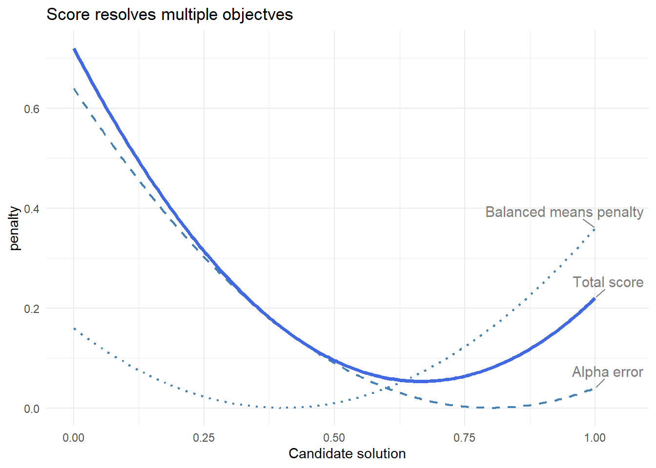
Interpreting the score function in Figure 1

Alpha error is minimised at one point
Balance penalty at another
The final score is a compromise

The algorithm solves a multi-objective optimisation problem

In Figure 1, the horizontal axis (“candidate solution”) represents a range of possible datasets that the algorithm might consider. Each point corresponds to a different arrangement of item values, with varying levels of reliability and balance. The vertical axis shows the penalty assigned by each component of the score function.

The curves illustrate how different criteria favour different solutions. The alpha error is lowest where the dataset is closest to the target Cronbach’s alpha, while the balance penalty is lowest where item means are most evenly distributed. These preferred solutions do not coincide. The total score combines both components, producing a compromise that reflects the relative weighting of each objective.

In practice, the algorithm moves through many such candidate solutions, using the score to evaluate their quality and guide the search toward an optimal balance.

Simulated Annealing: How We Search

Once we can evaluate solutions, we need a way to find good ones.

The problem with greedy search

A simple strategy:

Always accept improvements

A “greedy search” makes small changes and accepts every improvement, rejecting any changes that do not improve the configuration. An earlier version of the makeItemsScale() function did just this. It was fast, but often failed to converge to give the desired alpha value because the algorithm was trapped in a local minimum solution.

The idea of simulated annealing

Simulated annealing allows occasional “worse” moves.

Early: explore widely
Later: refine carefully

Temperature

At each step, worse moves are accepted with probability:

$P = exp ( \, - \frac {\Delta} {T} ) \,$

where:

$\Delta$ = how much worse the new solution is
$T$ = temperature

What this means

High temperature

$T$ is large
$\frac{\Delta} {T}$ is small
$exp ( - \frac {\Delta}{T} ) \approx 1$

Worse moves are often accepted

Low temperature

$T$ is small
$\frac{\Delta} {T}$ is large
$exp ( - \frac {\Delta}{T} ) \approx 0$

Worse moves are almost never accepted

High temperature → more exploration
Low temperature → more selective

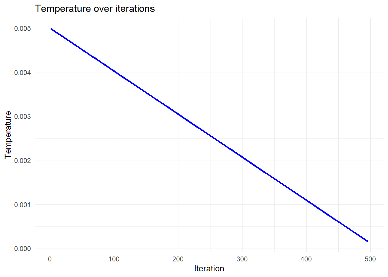
Temperature decreases over time:

Temperature “cools” over time

In this function, temperature starts at an initial value $T_0$ , and gradually decreases:

$T = T_0 * (1 - iter / max\_iter)$

Figure 2: Simulated Annealing temperature cooling over iterations

Visual intuition

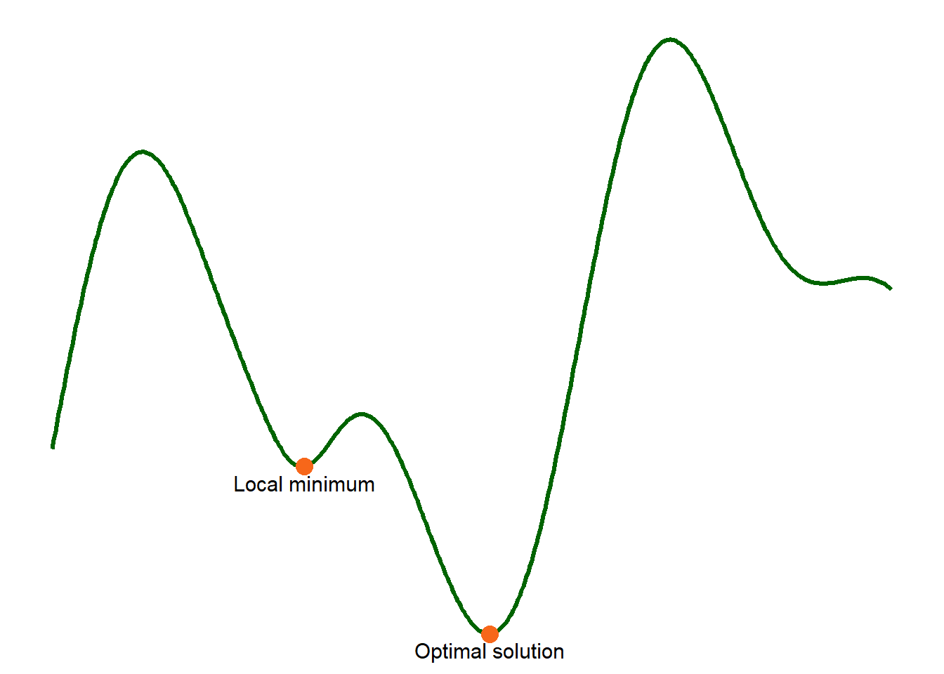
Figure 3: Notional search space for optimisation algorithm

Think of a landscape as in Figure 3:

Valleys = good solutions
Shallow valleys = local minima
Deepest valley = optimal solution

A greedy search gets stuck.

Simulated annealing can escape and find better regions.

Types of Moves

The algorithm modifies rows while preserving row sums.

Redistribution

$[3, 4, 2, 3] \rightarrow [4, 3, 2, 3]$

One value increases
Another decreases

Swap

$[3, 4, 2, 3] \rightarrow [3, 2, 4, 3]$

Values exchanged
No change in distribution

Key constraint

Row sums are always preserved

This ensures consistency with the input scale.

How It All Works Together

At each iteration:

Propose a change
Compute the score
Accept or reject based on temperature

The score defines the landscape; simulated annealing explores it.

What the Algorithm Looks Like in Practice

We can track the algorithm over time.

Temperature

Decreases steadily
Controls exploration

Score

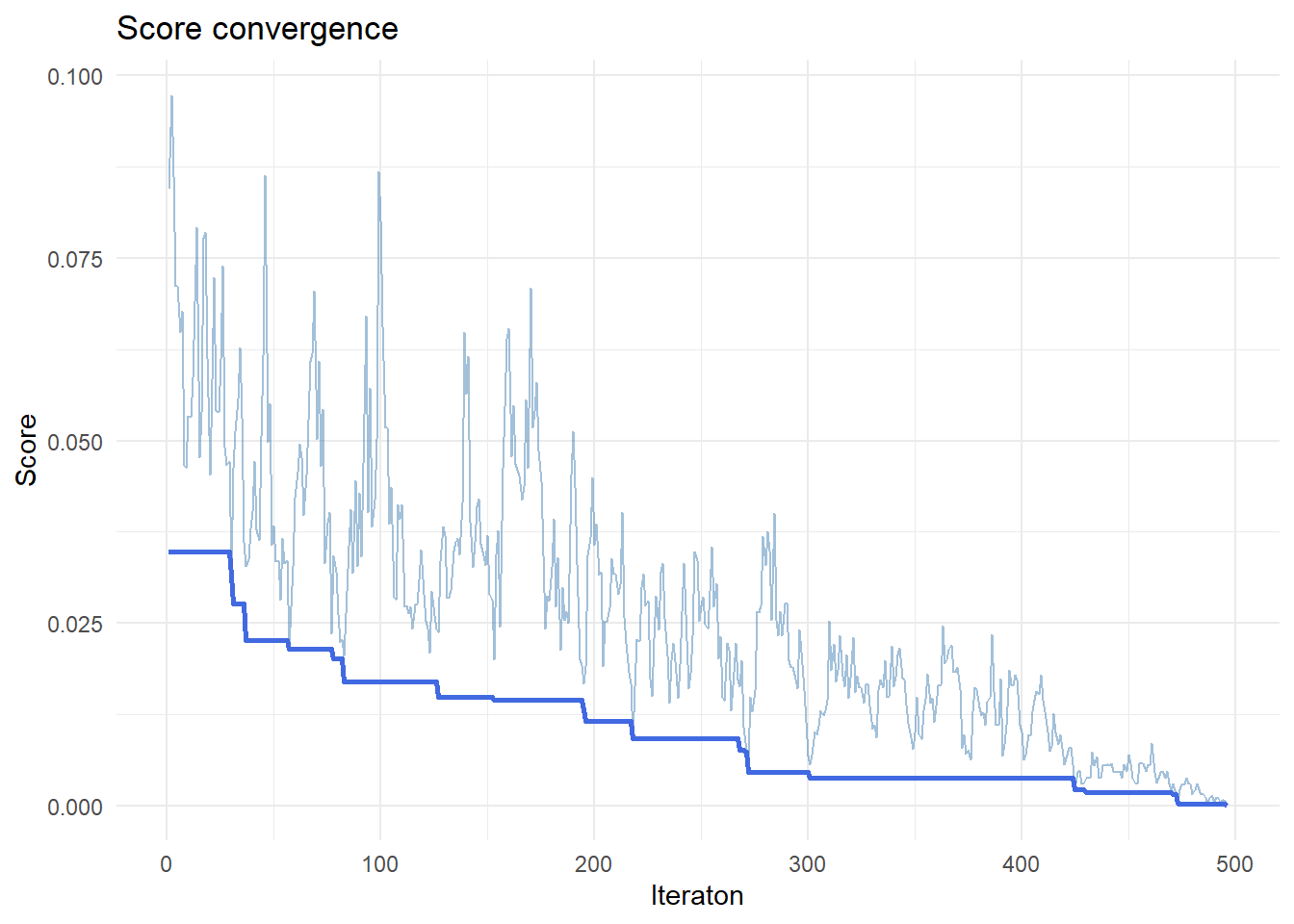
As we see in Figure 4:

Noisy early
Stabilises over time

The lighter line shows the current value for score at each iteration. The heavy line shows the best value achieved so far, improving steadily over time.

Early iterations have wide variation, reflecting exploration with high temperature. Later iterations have lower temperature and reduced variation.

Alpha

Figure 5 shows that over time, alpha:

Fluctuates early
Converges toward target

Convergence Toward Target Alpha

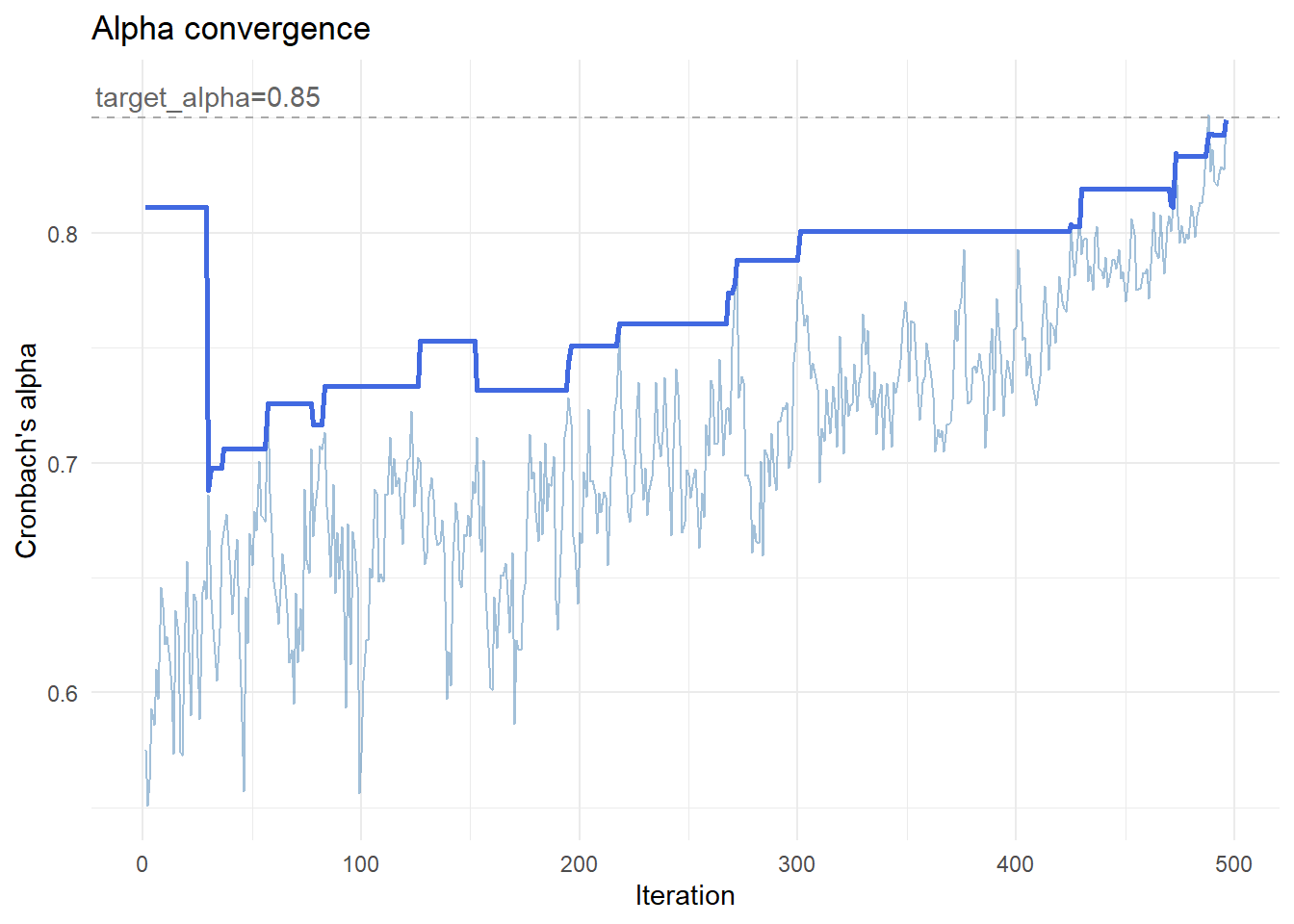
Figure 5: Simulated Annealing Cronbach’s alpha over iterations

The lighter line shows the current alpha, which fluctuates as the algorithm explores different configurations. The darker line tracks the best solution found so far, improving steadily over time.

Early iterations are volatile, reflecting exploration. Later iterations stabilise as the algorithm refines the solution.

This transition from exploration to refinement is the defining feature of simulated annealing.

Extensions

The score function can be extended to include:

variance constraints
distribution shape
additional structural properties

However:

More constraints make optimisation harder

Summary

The problem is to reconstruct item-level data from scale totals
The score function defines what “good” means
Simulated annealing enables effective search
The result is a flexible, realistic dataset with controlled reliability

item01	item02	item03	item04	X1	X2	X3	X4	summated_scale
4	4	3	3	3	3	4	4	14
3	3	2	3	3	2	3	3	11
3	3	1	3	3	3	3	1	10
2	5	3	3	4	4	3	2	13
5	4	3	5	4	4	4	5	17
4	5	4	5	5	4	5	4	18
4	4	2	3	3	3	4	3	13
4	3	3	3	3	3	3	4	13
4	3	4	4	3	4	4	4	15
3	3	2	4	3	3	2	4	12
2	2	1	3	2	2	2	2	8
2	2	2	3	3	2	2	2	9
4	5	3	4	4	4	5	3	16
5	4	3	3	3	4	4	4	15
4	4	2	3	3	3	3	4	13
5	4	5	4	5	5	3	5	18

item01	item02	item03	item04	X1	X2	X3	X4	summated_scale
4	4	3	3	3	3	4	4	14
3	3	2	3	3	2	3	3	11
3	3	1	3	3	3	3	1	10
2	5	3	3	4	4	3	2	13
5	4	3	5	4	4	4	5	17
4	5	4	5	5	4	5	4	18
4	4	2	3	3	3	4	3	13
4	3	3	3	3	3	3	4	13
4	3	4	4	3	4	4	4	15
3	3	2	4	3	3	2	4	12
2	2	1	3	2	2	2	2	8
2	2	2	3	3	2	2	2	9
4	5	3	4	4	4	5	3	16
5	4	3	3	3	4	4	4	15
4	4	2	3	3	3	3	4	13
5	4	5	4	5	5	3	5	18

item01	item02	item03	item04	X1	X2	X3	X4	summated_scale
4	4	3	3	3	3	4	4	14
3	3	2	3	3	2	3	3	11
3	3	1	3	3	3	3	1	10
2	5	3	3	4	4	3	2	13
5	4	3	5	4	4	4	5	17
4	5	4	5	5	4	5	4	18
4	4	2	3	3	3	4	3	13
4	3	3	3	3	3	3	4	13
4	3	4	4	3	4	4	4	15
3	3	2	4	3	3	2	4	12
2	2	1	3	2	2	2	2	8
2	2	2	3	3	2	2	2	9
4	5	3	4	4	4	5	3	16
5	4	3	3	3	4	4	4	15
4	4	2	3	3	3	3	4	13
5	4	5	4	5	5	3	5	18