LikertMakeR vignette

Hume Winzar

April 2025

LikertMakeR (Winzar, 2022) lets you create synthetic Likert-scale, or related rating-scale, data.
Set the mean, standard deviation, and correlations or model coefficients, and the package generates data matching those properties. It can also rearrange existing data columns to achieve a desired correlation structure or generate data based on Cronbach’s Alpha, factor correlations, regression or ANOVA coefficients, or other summary statistics.

Purpose

The package should be useful for teaching in the Social Sciences, and for scholars who wish to “replicate” or “reverse engineer” rating-scale data for further analysis and visualisation when only summary statistics have been reported.

Motivation

I was prompted to write the core functions in LikertMakeR after reviewing too many journal article submissions where authors presented questionnaire results with only means and standard deviations (often only the means), with no apparent understanding of scale distributions, and their impact on scale properties.

Hopefully, this tool will help researchers, teachers & students, and other reviewers, to better think about rating-scale distributions, and the effects of variance, scale boundaries, and number of items in a scale. Researchers can also use LikertMakeR to create dummy data to prepare analyses ahead of a formal survey.

Rating scale properties

A Likert scale is the mean, or sum, of several ordinal rating scales. Typically, they are bipolar (usually “agree-disagree”) responses to propositions that are determined to be moderately-to-highly correlated and that capture some facet of a theoretical construct.

Rating scales, such as Likert scales, are not continuous or unbounded.

For example, a 5-point Likert scale that is constructed with, say, five items (questions) will have a summed range of between 5 (all rated ‘1’) and 25 (all rated ‘5’) with all integers in between, and the mean range will be ‘1’ to ‘5’ with intervals of 1/5=0.20. A 7-point Likert scale constructed from eight items will have a summed range between 8 (all rated ‘1’) and 56 (all rated ‘7’) with all integers in between, and the mean range will be ‘1’ to ‘7’ with intervals of 1/8=0.125.

Technically, because they are bounded and not continuous, parametric statistics, such as mean, standard deviation, and correlation, should not be applied to summated rating scales. In practice, however, parametric statistics are commonly used in the social sciences because:

1. they are in common usage and easily understood,

2. results and conclusions drawn from technically-correct non-parametric statistics are (almost) always the same as for parametric statistics for such data.
   For example, D’Alessandro et al. (2020) argue that a summated scale, made with multiple items, “approaches” an interval scale measure, implying that parametric statistics are quite acceptable.

Rating-scale boundaries define minima and maxima for any scale values. If the mean is close to one boundary then data points will gather more closely to that boundary.
If the mean is not in the middle of a scale, then the data will be always skewed, as shown in the following plots.

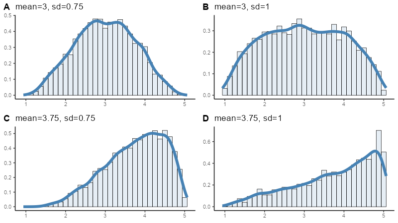
Off-centre means always give skewed distribution in bounded rating scales

---

LikertMakeR functions

• lfast() generate a vector of values with predefined mean and standard deviation.

• lcor() takes a dataframe of rating-scale values and rearranges the values in each column so that the columns are correlated to match a predefined correlation matrix.

• makeCorrAlpha constructs a random correlation matrix of given dimensions from a predefined Cronbach’s Alpha.

• makeCorrLoadings constructs a random correlation matrix from a given factor loadings matrix, and factor-correlations matrix.

• makeScales() is a wrapper function for lfast() and lcor() to generate items or summated scales with predefined first and second moments and a predefined correlation matrix. This function replaces makeItems() and now includes multi-item measures.

• makeItemsScale() generates a random dataframe of scale items based on a predefined summated scale with a desired Cronbach’s Alpha.

• makePaired() generates a dataframe of two correlated columns based on summary data from a paired-sample t-test.

• makeRepeated() generates a dataframe of ‘k’ correlated columns based on summary data from a repeated-samples ANOVA.

• makeScalesRegression() generates a dataframe based on results of output from multiple-regression - R², standardised betas, and IV correlations (if available).

• correlateScales() creates a dataframe of correlated summated scales as one might find in completed survey questionnaire and possibly used in a Structural Equation model.

• Helper Functions

  • alpha() calculates Cronbach’s Alpha from a given correlation matrix or a given dataframe.

  • eigenvalues() calculates eigenvalues of a correlation matrix, reports on positive-definite status of the matrix and, optionally, displays a scree plot to visualise the eigenvalues.

---

Using LikertMakeR

Download and Install LikertMakeR

from CRAN

> ```
>
> install.packages("LikertMakeR")
> library(LikertMakeR)
>
> ```

development version from GitHub.

> ```
> 
> library(devtools)
> install_github("WinzarH/LikertMakeR")
> library(LikertMakeR)
>
> ```

---

Generate synthetic rating-scale data

lfast()

• lfast() applies a simple evolutionary algorithm which draws repeated random samples from a scaled Beta distribution. It produces a vector of values with mean and standard deviation typically correct to two decimal places.

To synthesise a rating scale with lfast(), the user must input the following parameters:

• n: sample size

• mean: desired mean

• sd: desired standard deviation

• lowerbound: desired lower bound

• upperbound: desired upper bound

• items: number of items making the scale - default = 1

An earlier version of LikertMakeR had a function, lexact(), which was slow and no more accurate than the latest version of lfast(). So, lexact() is now deprecated.

lfast() example

a four-item, five-point Likert scale

nItems <- 4
mean <- 2.5
sd <- 0.75

x1 <- lfast(
  n = 512,
  mean = mean,
  sd = sd,
  lowerbound = 1,
  upperbound = 5,
  items = nItems
)
#> best solution in 256 iterations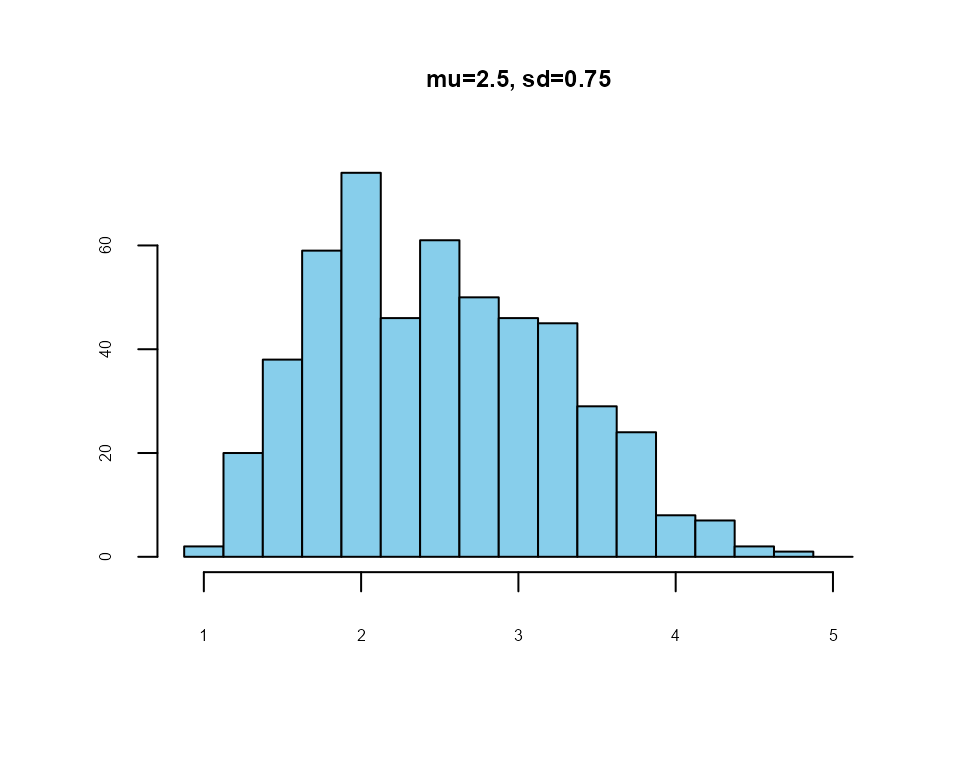

Example: 4-item, 1-5 Likert scale

an 11-point likelihood-of-purchase scale

lfast()

x2 <- lfast(256, 3, 2.5, 0, 10)
#> best solution in 7723 iterations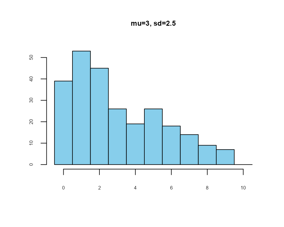

Example: likelihood-of-purchase scale

---

Correlating rating scales

The function, lcor(), rearranges the values in the columns of a data-set so that they are correlated at a specified level. It does not change the values - it swaps their positions within each column so that univariate statistics do not change, but their correlations with other vectors do.

lcor()

lcor() systematically selects pairs of values in a column and swaps their places, and checks to see if this swap improves the correlation matrix. If the revised dataframe produces a correlation matrix closer to the target correlation matrix, then the swap is retained. Otherwise, the values are returned to their original places. This process is iterated across each column.

To create the desired correlated data, the user must define the following parameters:

• data: a starter data set of rating-scales. Number of columns must match the dimensions of the target correlation matrix.

• target: the target correlation matrix.

lcor() example

Let’s generate some data: three 5-point Likert scales, each with five items.

## generate uncorrelated synthetic data
n <- 128
lowerbound <- 1
upperbound <- 5
items <- 5

mydat3 <- data.frame(
  x1 = lfast(n, 2.5, 0.75, lowerbound, upperbound, items),
  x2 = lfast(n, 3.0, 1.50, lowerbound, upperbound, items),
  x3 = lfast(n, 3.5, 1.00, lowerbound, upperbound, items)
)
#> best solution in 812 iterations
#> best solution in 7553 iterations
#> best solution in 385 iterations

The first six observations from this dataframe are:

#>    x1  x2  x3
#> 1 1.4 1.0 5.0
#> 2 2.8 5.0 4.2
#> 3 3.4 1.8 2.0
#> 4 2.0 4.8 4.4
#> 5 3.6 1.0 3.4
#> 6 2.2 2.8 4.0

And the first and second moments (to 3 decimal places) are:

#>         x1    x2    x3
#> mean 2.500 3.002 3.498
#> sd   0.752 1.501 1.001

We can see that the data have first and second moments are very close to what is expected.

As we should expect, randomly-generated synthetic data have low correlations:

#>       x1    x2   x3
#> x1  1.00 -0.02 0.03
#> x2 -0.02  1.00 0.00
#> x3  0.03  0.00 1.00

Now, let’s define a target correlation matrix:

## describe a target correlation matrix
tgt3 <- matrix(
  c(
    1.00, 0.85, 0.75,
    0.85, 1.00, 0.65,
    0.75, 0.65, 1.00
  ),
  nrow = 3
)

So now we have a dataframe with desired first and second moments, and a target correlation matrix.

## apply lcor() function
new3 <- lcor(data = mydat3, target = tgt3)

Values in each column of the new dataframe do not change from the original; the values are rearranged.

The first ten observations from this dataframe are:

#>     X1  X2  X3
#> 1  2.4 1.8 4.6
#> 2  3.4 5.0 4.0
#> 3  1.6 1.0 2.0
#> 4  2.8 4.8 4.2
#> 5  3.2 3.2 4.6
#> 6  2.4 2.8 4.0
#> 7  2.2 2.0 3.4
#> 8  3.2 4.6 4.8
#> 9  1.4 1.8 4.4
#> 10 3.0 4.8 4.2

And the new dataframe is correlated close to our desired correlation matrix; here presented to 3 decimal places:

#>      X1   X2   X3
#> X1 1.00 0.85 0.75
#> X2 0.85 1.00 0.65
#> X3 0.75 0.65 1.00

---

Generate a correlation matrix from Cronbach’s Alpha

makeCorrAlpha()

makeCorrAlpha(), constructs a random correlation matrix of given dimensions and predefined Cronbach’s Alpha.

To create the desired correlation matrix, the user must define the following parameters:

• items: or “k” - the number of rows and columns of the desired correlation matrix.

• alpha: the target value for Cronbach’s Alpha

• variance: a notional variance coefficient to affect the spread of values in the correlation matrix. Default = ‘0.5’. A value of ‘0’ produces a matrix where all off-diagonal correlations are equal. Setting ‘variance = 1.0’ gives a wider range of values. Setting ‘variance = 2.0’, or above, may be feasible but increases the likelihood of a non-positive-definite matrix.

• precision: a value between ‘0’ and ‘3’ to add some random variation around the target Cronbach’s Alpha. Default = ‘0’. A value of ‘0’ produces the desired Alpha, generally exact to two decimal places. Higher values produce increasingly random values around the desired Alpha.

• sort_cors: Logical. Default = FALSE. If TRUE, then runs more quickly, but produces a less natural correlation matrix.

• diagnostics: Logical. If TRUE, returns a list containing the correlation matrix and a diagnostics list (target/achieved alpha, average inter-item correlation, eigenvalues, PD flag, and key arguments). If FALSE (default), returns the correlation matrix only.

makeCorrAlpha() is volatile

Random values generated by makeCorrAlpha() are highly volatile. makeCorrAlpha() may not generate a feasible (positive-definite) correlation matrix, especially when

• variance is high relative to

  • desired Alpha, and
  • desired correlation dimensions

makeCorrAlpha() will inform the user if the resulting correlation matrix is positive definite, or not.

If the returned correlation matrix is not positive-definite, a feasible solution may be still possible, and often is. The user is encouraged to try again, possibly several times, to find one.

makeCorrAlpha() examples

Four variables, alpha = 0.85, variance = default

## define parameters
items <- 4
alpha <- 0.85
# variance <- 0.5 ## by default

## apply makeCorrAlpha() function
set.seed(42)

cor_matrix_4 <- makeCorrAlpha(items, alpha)
#> correlation values consistent with desired alpha in 59 iterations

makeCorrAlpha() produced the following correlation matrix (to three decimal places):

#>        item01 item02 item03 item04
#> item01  1.000  0.766  0.693  0.433
#> item02  0.766  1.000  0.694  0.425
#> item03  0.693  0.694  1.000  0.507
#> item04  0.433  0.425  0.507  1.000

test output with Helper functions

## using helper function alpha()

alpha(cor_matrix_4)
#> [1] 0.8500063

## using helper function eigenvalues()

eigenvalues(cor_matrix_4, 1)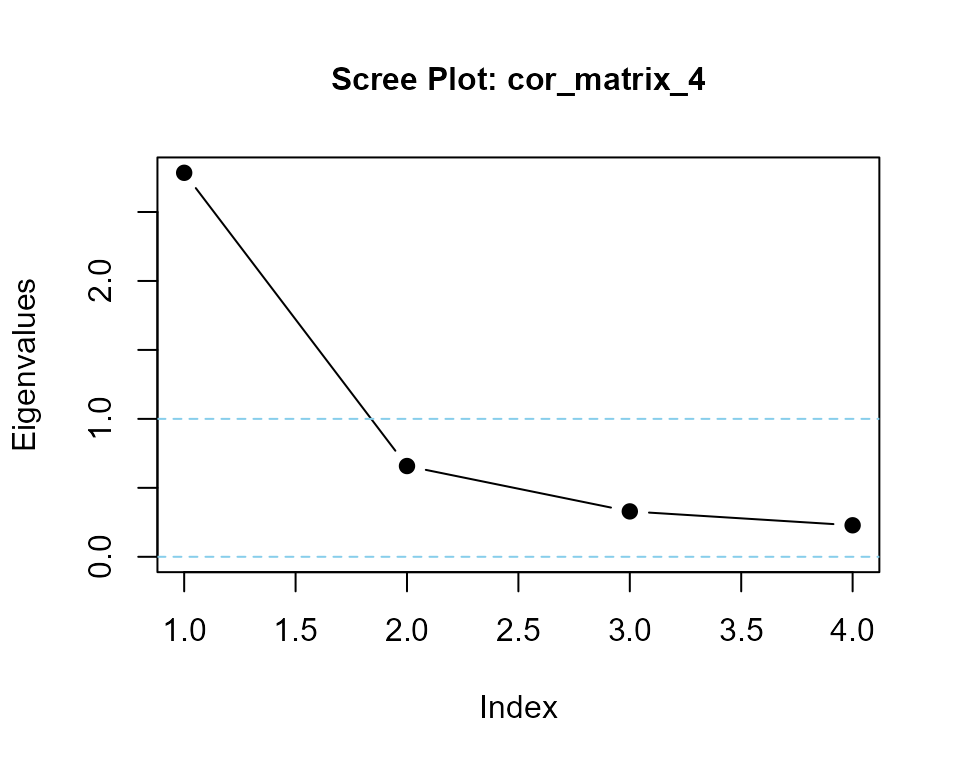

#> cor_matrix_4  is positive-definite
#> [1] 2.7831667 0.6670820 0.3157114 0.2340400

twelve variables, alpha = 0.90, variance = 1

## define parameters
items <- 12
alpha <- 0.90
variance <- 1.0

## apply makeCorrAlpha() function
set.seed(42)

cor_matrix_12 <- makeCorrAlpha(items = items, alpha = alpha, variance = variance)
#> correlation values consistent with desired alpha in 4312 iterations
#> Correlation matrix is not yet positive definite
#> Working on it
#> 
#> improved at swap - 1 (min eigenvalue: -0.953206)
#> improved at swap - 4 (min eigenvalue: -0.948513)
#> improved at swap - 7 (min eigenvalue: -0.885627)
#> improved at swap - 11 (min eigenvalue: -0.823701)
#> improved at swap - 13 (min eigenvalue: -0.817121)
#> improved at swap - 18 (min eigenvalue: -0.795548)
#> improved at swap - 19 (min eigenvalue: -0.786689)
#> improved at swap - 24 (min eigenvalue: -0.785326)
#> improved at swap - 25 (min eigenvalue: -0.783145)
#> improved at swap - 30 (min eigenvalue: -0.780524)
#> improved at swap - 33 (min eigenvalue: -0.770617)
#> improved at swap - 43 (min eigenvalue: -0.769144)
#> improved at swap - 47 (min eigenvalue: -0.76871)
#> improved at swap - 49 (min eigenvalue: -0.767956)
#> improved at swap - 74 (min eigenvalue: -0.75443)
#> improved at swap - 84 (min eigenvalue: -0.709321)
#> improved at swap - 89 (min eigenvalue: -0.709319)
#> improved at swap - 97 (min eigenvalue: -0.709101)
#> improved at swap - 105 (min eigenvalue: -0.702808)
#> improved at swap - 109 (min eigenvalue: -0.686501)
#> improved at swap - 123 (min eigenvalue: -0.675567)
#> improved at swap - 149 (min eigenvalue: -0.656166)
#> improved at swap - 154 (min eigenvalue: -0.647445)
#> improved at swap - 156 (min eigenvalue: -0.639865)
#> improved at swap - 162 (min eigenvalue: -0.636826)
#> improved at swap - 207 (min eigenvalue: -0.636473)
#> improved at swap - 227 (min eigenvalue: -0.631569)
#> improved at swap - 239 (min eigenvalue: -0.631529)
#> improved at swap - 260 (min eigenvalue: -0.630315)
#> improved at swap - 265 (min eigenvalue: -0.630018)
#> improved at swap - 277 (min eigenvalue: -0.628351)
#> improved at swap - 305 (min eigenvalue: -0.624799)
#> improved at swap - 306 (min eigenvalue: -0.620084)
#> improved at swap - 330 (min eigenvalue: -0.61767)
#> improved at swap - 370 (min eigenvalue: -0.616984)
#> improved at swap - 410 (min eigenvalue: -0.615695)
#> improved at swap - 413 (min eigenvalue: -0.610777)
#> improved at swap - 432 (min eigenvalue: -0.609952)
#> improved at swap - 454 (min eigenvalue: -0.609934)
#> improved at swap - 464 (min eigenvalue: -0.608802)
#> improved at swap - 475 (min eigenvalue: -0.606048)
#> improved at swap - 480 (min eigenvalue: -0.604196)
#> improved at swap - 481 (min eigenvalue: -0.603605)
#> improved at swap - 489 (min eigenvalue: -0.603575)
#> improved at swap - 509 (min eigenvalue: -0.557319)
#> improved at swap - 517 (min eigenvalue: -0.556993)
#> improved at swap - 525 (min eigenvalue: -0.555728)
#> improved at swap - 550 (min eigenvalue: -0.550725)
#> improved at swap - 584 (min eigenvalue: -0.546519)
#> improved at swap - 588 (min eigenvalue: -0.54343)
#> improved at swap - 589 (min eigenvalue: -0.525605)
#> improved at swap - 609 (min eigenvalue: -0.520762)
#> improved at swap - 677 (min eigenvalue: -0.520203)
#> improved at swap - 682 (min eigenvalue: -0.517845)
#> improved at swap - 735 (min eigenvalue: -0.517013)
#> improved at swap - 772 (min eigenvalue: -0.516949)
#> improved at swap - 823 (min eigenvalue: -0.516743)
#> improved at swap - 840 (min eigenvalue: -0.516391)
#> improved at swap - 848 (min eigenvalue: -0.512467)
#> improved at swap - 852 (min eigenvalue: -0.512226)
#> improved at swap - 896 (min eigenvalue: -0.512095)
#> improved at swap - 911 (min eigenvalue: -0.51205)
#> improved at swap - 916 (min eigenvalue: -0.51194)
#> improved at swap - 917 (min eigenvalue: -0.510744)
#> improved at swap - 969 (min eigenvalue: -0.509389)
#> improved at swap - 971 (min eigenvalue: -0.508507)
#> improved at swap - 974 (min eigenvalue: -0.508265)
#> improved at swap - 1000 (min eigenvalue: -0.501376)
#> improved at swap - 1006 (min eigenvalue: -0.500307)
#> improved at swap - 1024 (min eigenvalue: -0.49485)
#> improved at swap - 1084 (min eigenvalue: -0.494849)
#> improved at swap - 1114 (min eigenvalue: -0.49467)
#> improved at swap - 1127 (min eigenvalue: -0.492862)
#> improved at swap - 1138 (min eigenvalue: -0.491828)
#> improved at swap - 1146 (min eigenvalue: -0.488759)
#> improved at swap - 1220 (min eigenvalue: -0.487876)
#> improved at swap - 1230 (min eigenvalue: -0.487867)
#> improved at swap - 1235 (min eigenvalue: -0.48684)
#> improved at swap - 1299 (min eigenvalue: -0.486493)
#> improved at swap - 1413 (min eigenvalue: -0.482833)
#> improved at swap - 1434 (min eigenvalue: -0.48144)
#> improved at swap - 1534 (min eigenvalue: -0.481217)
#> improved at swap - 1538 (min eigenvalue: -0.481094)
#> improved at swap - 1637 (min eigenvalue: -0.479178)
#> improved at swap - 1647 (min eigenvalue: -0.478561)
#> improved at swap - 1704 (min eigenvalue: -0.476757)
#> improved at swap - 1780 (min eigenvalue: -0.474676)
#> improved at swap - 1806 (min eigenvalue: -0.474662)
#> improved at swap - 1953 (min eigenvalue: -0.474644)
#> improved at swap - 1956 (min eigenvalue: -0.474581)
#> improved at swap - 1984 (min eigenvalue: -0.47448)
#> improved at swap - 2006 (min eigenvalue: -0.474466)
#> improved at swap - 2016 (min eigenvalue: -0.470122)
#> improved at swap - 2034 (min eigenvalue: -0.468171)
#> improved at swap - 2326 (min eigenvalue: -0.468064)
#> improved at swap - 2338 (min eigenvalue: -0.467538)
#> improved at swap - 2350 (min eigenvalue: -0.467353)
#> improved at swap - 2435 (min eigenvalue: -0.466742)
#> improved at swap - 2487 (min eigenvalue: -0.466487)
#> improved at swap - 2516 (min eigenvalue: -0.465717)
#> improved at swap - 2522 (min eigenvalue: -0.465611)
#> improved at swap - 2535 (min eigenvalue: -0.460623)
#> improved at swap - 2576 (min eigenvalue: -0.460212)
#> improved at swap - 2678 (min eigenvalue: -0.460061)
#> improved at swap - 2761 (min eigenvalue: -0.458568)
#> improved at swap - 2795 (min eigenvalue: -0.458554)
#> improved at swap - 2827 (min eigenvalue: -0.458226)
#> improved at swap - 2832 (min eigenvalue: -0.458215)
#> improved at swap - 2838 (min eigenvalue: -0.456188)
#> improved at swap - 2934 (min eigenvalue: -0.455385)
#> improved at swap - 2948 (min eigenvalue: -0.455052)
#> improved at swap - 3114 (min eigenvalue: -0.454904)
#> improved at swap - 3171 (min eigenvalue: -0.454781)
#> improved at swap - 3175 (min eigenvalue: -0.454779)
#> improved at swap - 3384 (min eigenvalue: -0.454773)
#> improved at swap - 3425 (min eigenvalue: -0.454728)
#> improved at swap - 3768 (min eigenvalue: -0.454533)
#> improved at swap - 3994 (min eigenvalue: -0.454355)
#> improved at swap - 4095 (min eigenvalue: -0.454326)
#> improved at swap - 4123 (min eigenvalue: -0.45431)
#> improved at swap - 4141 (min eigenvalue: -0.454307)
#> improved at swap - 4202 (min eigenvalue: -0.453472)
#> improved at swap - 4241 (min eigenvalue: -0.453251)
#> improved at swap - 4396 (min eigenvalue: -0.452216)
#> improved at swap - 4584 (min eigenvalue: -0.452049)
#> improved at swap - 4598 (min eigenvalue: -0.451984)
#> improved at swap - 4811 (min eigenvalue: -0.451936)
#> improved at swap - 4887 (min eigenvalue: -0.451751)
#> improved at swap - 4900 (min eigenvalue: -0.451602)
#> improved at swap - 5158 (min eigenvalue: -0.451459)
#> improved at swap - 5182 (min eigenvalue: -0.451271)
#> improved at swap - 5225 (min eigenvalue: -0.45124)
#> improved at swap - 5660 (min eigenvalue: -0.451226)
#> improved at swap - 5947 (min eigenvalue: -0.450989)
#> improved at swap - 5955 (min eigenvalue: -0.450651)
#> improved at swap - 5981 (min eigenvalue: -0.450623)
#> improved at swap - 6020 (min eigenvalue: -0.450603)
#> improved at swap - 6486 (min eigenvalue: -0.450145)
#> improved at swap - 7033 (min eigenvalue: -0.44951)
#> improved at swap - 7251 (min eigenvalue: -0.44897)
#> improved at swap - 7284 (min eigenvalue: -0.448929)
#> improved at swap - 7422 (min eigenvalue: -0.448928)
#> improved at swap - 7491 (min eigenvalue: -0.448854)
#> improved at swap - 7804 (min eigenvalue: -0.448834)
#> improved at swap - 7830 (min eigenvalue: -0.448833)
#> improved at swap - 7996 (min eigenvalue: -0.448577)
#> improved at swap - 8059 (min eigenvalue: -0.448564)
#> improved at swap - 8082 (min eigenvalue: -0.448492)
#> improved at swap - 8300 (min eigenvalue: -0.448205)
#> improved at swap - 8360 (min eigenvalue: -0.448158)
#> improved at swap - 8384 (min eigenvalue: -0.447955)
#> improved at swap - 8538 (min eigenvalue: -0.447952)
#> improved at swap - 8672 (min eigenvalue: -0.447944)
#> improved at swap - 8803 (min eigenvalue: -0.447936)
#> improved at swap - 9042 (min eigenvalue: -0.447897)
#> improved at swap - 9100 (min eigenvalue: -0.447875)
#> improved at swap - 9335 (min eigenvalue: -0.447862)
#> improved at swap - 9436 (min eigenvalue: -0.447824)
#> improved at swap - 9585 (min eigenvalue: -0.447823)
#> improved at swap - 10072 (min eigenvalue: -0.447799)
#> improved at swap - 10797 (min eigenvalue: -0.447797)
#> improved at swap - 11139 (min eigenvalue: -0.447796)
#> improved at swap - 11305 (min eigenvalue: -0.447777)
#> improved at swap - 11878 (min eigenvalue: -0.447767)
#> improved at swap - 12608 (min eigenvalue: -0.447766)
#> improved at swap - 14464 (min eigenvalue: -0.447756)
#> stopped after 158213 swaps (no improvement for 143748 attempts)

-

makeCorrAlpha() produced the following correlation matrix (to two decimal places):

#>        item01 item02 item03 item04 item05 item06 item07 item08 item09 item10
#> item01   1.00  -0.07   0.57  -0.51   0.81   0.56   0.61  -0.27   0.43   0.31
#> item02  -0.07   1.00   0.53   0.88   0.56   0.47  -0.04   0.62   0.70   0.34
#> item03   0.57   0.53   1.00   0.33   0.79   0.39   0.62   0.83   0.46   0.62
#> item04  -0.51   0.88   0.33   1.00   0.70   0.62  -0.32   0.70   0.63   0.06
#> item05   0.81   0.56   0.79   0.70   1.00   0.70   0.60   0.26   0.79   0.06
#> item06   0.56   0.47   0.39   0.62   0.70   1.00  -0.67  -0.03   0.57   0.20
#> item07   0.61  -0.04   0.62  -0.32   0.60  -0.67   1.00   0.47   0.00   0.45
#> item08  -0.27   0.62   0.83   0.70   0.26  -0.03   0.47   1.00   0.36   0.89
#> item09   0.43   0.70   0.46   0.63   0.79   0.57   0.00   0.36   1.00  -0.30
#> item10   0.31   0.34   0.62   0.06   0.06   0.20   0.45   0.89  -0.30   1.00
#> item11   0.66   0.36   0.97   0.26   0.84   0.25   0.78   0.80   0.72   0.48
#> item12   0.50  -0.29   0.71   0.28   0.73   0.42   0.59   0.64  -0.14   0.72
#>        item11 item12
#> item01   0.66   0.50
#> item02   0.36  -0.29
#> item03   0.97   0.71
#> item04   0.26   0.28
#> item05   0.84   0.73
#> item06   0.25   0.42
#> item07   0.78   0.59
#> item08   0.80   0.64
#> item09   0.72  -0.14
#> item10   0.48   0.72
#> item11   1.00   0.71
#> item12   0.71   1.00

test output

## calculate Cronbach's Alpha
alpha(cor_matrix_12)
#> [1] 0.9000045

## calculate eigenvalues of the correlation matrix
eigenvalues(cor_matrix_12, 1) |> round(3)

#> cor_matrix_12  is NOT positive-definite
#>  [1]  6.033  3.006  2.192  1.396  0.789  0.371  0.081 -0.169 -0.364 -0.441
#> [11] -0.447 -0.448

makeCorrAlpha() with diagnostics output

## apply makeCorrAlpha() with diagnostics
set.seed(42)

cor_matrix_5 <- makeCorrAlpha(
  items = 6,
  alpha = 0.90,
  diagnostics = TRUE
)
#> reached max iterations (3600) - best mean difference: 3.2e-05
#> Correlation matrix is not yet positive definite
#> Working on it
#> 
#> improved at swap - 2 (min eigenvalue: -0.059282)
#> improved at swap - 3 (min eigenvalue: -0.047945)
#> improved at swap - 4 (min eigenvalue: -0.010881)
#> improved at swap - 6 (min eigenvalue: 0.023082)
#> positive definite at swap - 6

diagnostics output

## output
cor_matrix_5$R |> round(2)
#>        item01 item02 item03 item04 item05 item06
#> item01   1.00   0.70   0.63   0.83   0.75   0.74
#> item02   0.70   1.00   0.31   0.53   0.51   0.44
#> item03   0.63   0.31   1.00   0.49   0.79   0.73
#> item04   0.83   0.53   0.49   1.00   0.64   0.36
#> item05   0.75   0.51   0.79   0.64   1.00   0.55
#> item06   0.74   0.44   0.73   0.36   0.55   1.00

cor_matrix_5$diagnostics
#> $items
#> [1] 6
#> 
#> $alpha_target
#> [1] 0.9
#> 
#> $alpha_achieved
#> [1] 0.90002
#> 
#> $average_r
#> [1] 0.6000534
#> 
#> $eigenvalues
#> [1] 4.03582074 0.86126219 0.58519829 0.35723432 0.13740248 0.02308198
#> 
#> $is_positive_definite
#> [1] TRUE
#> 
#> $variance
#> [1] 0.5
#> 
#> $precision
#> [1] 0
#> 
#> $sort_cors
#> [1] FALSE

---

Generate a correlation matrix from factor loadings

makeCorrLoadings

makeCorrLoadings() generates a correlation matrix from factor loadings and factor correlations as might be seen in Exploratory Factor Analysis (EFA) or a Structural Equation Model (SEM).

makeCorrLoadings() usage

  makeCorrLoadings(loadings, factorCor = NULL, uniquenesses = NULL, nearPD = FALSE)

makeCorrLoadings() arguments

• loadings: ‘k’ (items) by ‘f’ (factors) matrix of standardised factor loadings. Item names and Factor names can be taken from the row_names (items) and the column_names (factors), if present.

• factorCor: ‘f’ x ‘f’ factor correlation matrix. If not present, then we assume that the factors are uncorrelated (orthogonal), which is rare in practice, and the function applies an identity matrix for factor_cor.

• uniquenesses: length ‘k’ vector of uniquenesses. If NULL, the default, compute from the calculated communalities.

• nearPD: (logical) If TRUE, then the function calls the nearPD function from the Matrix package to transform the resulting correlation matrix onto the nearest Positive Definite matrix. Obviously, this only applies if the resulting correlation matrix is not positive definite. (It should never be needed.)

Note

“Censored” loadings (for example, where loadings less than some small value (often ‘0.30’), are removed for ease-of-communication) tend to severely reduce the accuracy of the makeCorrLoadings() function. For a detailed demonstration, see the vignette file, makeCorrLoadings_Validate.

makeCorrLoadings() examples

Typical application from published EFA results

define parameters

## Example loadings

factorLoadings <- matrix(
  c(
    0.05, 0.20, 0.70,
    0.10, 0.05, 0.80,
    0.05, 0.15, 0.85,
    0.20, 0.85, 0.15,
    0.05, 0.85, 0.10,
    0.10, 0.90, 0.05,
    0.90, 0.15, 0.05,
    0.80, 0.10, 0.10
  ),
  nrow = 8, ncol = 3, byrow = TRUE
)

## row and column names

rownames(factorLoadings) <- c("Q1", "Q2", "Q3", "Q4", "Q5", "Q6", "Q7", "Q8")
colnames(factorLoadings) <- c("Factor1", "Factor2", "Factor3")

## Factor correlation matrix**

factorCor <- matrix(
  c(
    1.0,  0.5, 0.4,
    0.5,  1.0, 0.3,
    0.4,  0.3, 1.0
  ),
  nrow = 3, byrow = TRUE
)

Apply the function

## apply makeCorrLoadings() function
itemCorrelations <- makeCorrLoadings(factorLoadings, factorCor)

## derived correlation matrix to two decimal places
round(itemCorrelations, 2)
#>      Q1   Q2   Q3   Q4   Q5   Q6   Q7   Q8
#> Q1 1.00 0.62 0.67 0.48 0.42 0.42 0.43 0.41
#> Q2 0.62 1.00 0.72 0.43 0.36 0.36 0.44 0.42
#> Q3 0.67 0.72 1.00 0.50 0.43 0.43 0.46 0.45
#> Q4 0.48 0.43 0.50 1.00 0.79 0.83 0.65 0.58
#> Q5 0.42 0.36 0.43 0.79 1.00 0.80 0.54 0.48
#> Q6 0.42 0.36 0.43 0.83 0.80 1.00 0.59 0.52
#> Q7 0.43 0.44 0.46 0.65 0.54 0.59 1.00 0.78
#> Q8 0.41 0.42 0.45 0.58 0.48 0.52 0.78 1.00

Test makeCorrLoadings() output

## correlated factors mean that eigenvalues should suggest two or three factors
eigenvalues(cormatrix = itemCorrelations, scree = TRUE)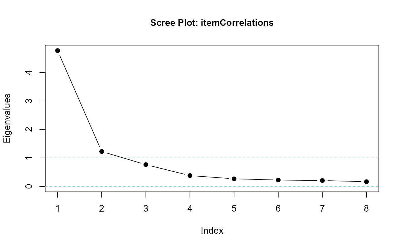

#> itemCorrelations  is positive-definite
#> [1] 4.7679427 1.2254239 0.7641967 0.3799863 0.2668158 0.2237851 0.2073574
#> [8] 0.1644922

Assuming orthogonal factors

## orthogonal factors are assumed when factor correlation matrix is not included
orthogonalItemCors <- makeCorrLoadings(factorLoadings)

## derived correlation matrix to two decimal places
round(orthogonalItemCors, 2)
#>      Q1   Q2   Q3   Q4   Q5   Q6   Q7   Q8
#> Q1 1.00 0.58 0.63 0.28 0.24 0.22 0.11 0.13
#> Q2 0.58 1.00 0.69 0.18 0.13 0.10 0.14 0.17
#> Q3 0.63 0.69 1.00 0.26 0.22 0.18 0.11 0.14
#> Q4 0.28 0.18 0.26 1.00 0.75 0.79 0.32 0.26
#> Q5 0.24 0.13 0.22 0.75 1.00 0.78 0.18 0.14
#> Q6 0.22 0.10 0.18 0.79 0.78 1.00 0.23 0.18
#> Q7 0.11 0.14 0.11 0.32 0.18 0.23 1.00 0.74
#> Q8 0.13 0.17 0.14 0.26 0.14 0.18 0.74 1.00

Test orthogonal output

## eigenvalues should suggest exactly  three factors
eigenvalues(cormatrix = orthogonalItemCors, scree = TRUE)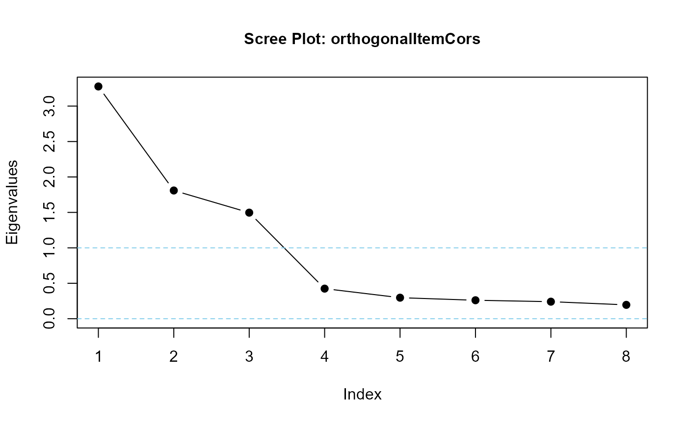

#> orthogonalItemCors  is positive-definite
#> [1] 3.2769426 1.8091128 1.4966064 0.4244753 0.2966222 0.2605233 0.2402622
#> [8] 0.1954553

---

Generate a dataframe of rating scales from a correlation matrix and predefined moments

makeScales()

makeScales() generates a dataframe of random discrete values so the data replicate a set of scale items or summated rating scales, and are correlated close to a predefined correlation matrix.

Generally, means, standard deviations, and correlations are correct to two decimal places.

makeScales() is a wrapper function for

• lfast(), which takes repeated samples selecting a vector that best fits the desired moments, and

• lcor(), which rearranges values in each column of the dataframe so they closely match the desired correlation matrix.

To create the desired dataframe, the user must define the following parameters:

• n: number of observations

• dfMeans: a vector of length ‘k’ of desired means of each variable

• dfSds: a vector of length ‘k’ of desired standard deviations of each variable

• lowerbound: a vector of length ‘k’ of values for the lower bound of each variable. default = ‘1’

• upperbound: a vector of length ‘k’ of values for the upper bound of each variable. Default = ‘5’

• items: a vector of length ‘k’ of the number of items in each variable. Default = ‘1’.

• cormatrix: a target correlation matrix with ‘k’ rows and ‘k’ columns.

makeScales() examples

four correlated items

## define parameters
n <- 128
dfMeans <- c(2.5, 3.0, 3.0, 3.5)
dfSds <- c(1.0, 1.0, 1.5, 0.75)
lowerbound <- rep(1, 4)
upperbound <- rep(5, 4)

corMat <- matrix(
  c(
    1.00, 0.25, 0.35, 0.45,
    0.25, 1.00, 0.70, 0.75,
    0.35, 0.70, 1.00, 0.85,
    0.45, 0.75, 0.85, 1.00
  ),
  nrow = 4, ncol = 4
)

var_names <- c("var1", "var2", "var3", "var4")
colnames(corMat) <- var_names
rownames(corMat) <- var_names

## apply makeScales() function
df <- makeScales(
  n = n,
  means = dfMeans,
  sds = dfSds,
  lowerbound = lowerbound,
  upperbound = upperbound,
  cormatrix = corMat
)
#> Variable  1 :  var1  -
#> reached maximum of 16384 iterations
#> Variable  2 :  var2  -
#> reached maximum of 16384 iterations
#> Variable  3 :  var3  -
#> best solution in 323 iterations
#> Variable  4 :  var4  -
#> reached maximum of 16384 iterations
#> 
#> Arranging data to match correlations
#> 
#> Successfully generated correlated variables

## test the function
str(df)
#> 'data.frame':    128 obs. of  4 variables:
#>  $ var1: num  1 3 1 4 5 4 2 3 2 3 ...
#>  $ var2: num  4 4 4 3 4 5 5 4 2 1 ...
#>  $ var3: num  5 4 5 3 5 5 4 5 2 2 ...
#>  $ var4: num  4 4 4 4 4 5 4 5 3 3 ...

### means should be correct to two decimal places
dfmoments <- data.frame(
  mean = apply(df, 2, mean) |> round(3),
  sd = apply(df, 2, sd) |> round(3)
) |> t()

dfmoments
#>       var1  var2  var3  var4
#> mean 2.500 3.000 3.000 3.500
#> sd   1.004 1.004 1.501 0.753

### correlations should be correct to two decimal places
cor(df) |> round(3)
#>       var1 var2  var3  var4
#> var1 1.000 0.25 0.350 0.448
#> var2 0.250 1.00 0.700 0.750
#> var3 0.350 0.70 1.000 0.843
#> var4 0.448 0.75 0.843 1.000

four Likert scales

Brand Trust (BT) - The confidence a consumer has in a brand’s reliability and honesty. Brand Satisfaction (BS) - Overall affective evaluation of the brand experience. Brand Love (BL) - Deep emotional attachment toward the brand. Brand Loyalty (BLY) - Intention to repurchase and recommend the brand.

## define parameters
n <- 256
dfMeans <- c(3.9, 4.1, 3.6, 4.0)
dfSds <- c(0.6, 0.5, 0.8, 0.7)
lowerbound <- rep(1, 4)
upperbound <- rep(5, 4)
items <- c(4, 3, 4, 3)

corMat <- matrix(
  c(
    1.00, 0.75, 0.60, 0.70,
    0.75, 1.00, 0.65, 0.72,
    0.60, 0.65, 1.00, 0.68,
    0.70, 0.72, 0.68, 1.00
  ),
  nrow = 4, ncol = 4
)

scale_names <- c("BT", "BS", "BL", "BLY")
rownames(corMat) <- scale_names
colnames(corMat) <- scale_names

## apply makeScales() function
df <- makeScales(
  n = n,
  means = dfMeans,
  sds = dfSds,
  lowerbound = lowerbound,
  upperbound = upperbound,
  items = items,
  cormatrix = corMat
)
#> Variable  1 :  BT  -
#> best solution in 336 iterations
#> Variable  2 :  BS  -
#> best solution in 421 iterations
#> Variable  3 :  BL  -
#> best solution in 923 iterations
#> Variable  4 :  BLY  -
#> best solution in 27 iterations
#> 
#> Arranging data to match correlations
#> 
#> Successfully generated correlated variables

## test the function
head(df)
#>     BT       BS   BL      BLY
#> 1 4.00 4.333333 3.75 4.666667
#> 2 2.25 3.666667 3.75 3.333333
#> 3 4.25 4.333333 3.75 4.666667
#> 4 4.00 3.333333 3.00 4.333333
#> 5 3.75 4.333333 4.00 4.333333
#> 6 4.50 4.666667 4.50 5.000000
tail(df)
#>       BT       BS   BL      BLY
#> 251 3.75 4.000000 3.75 4.000000
#> 252 4.75 5.000000 4.00 5.000000
#> 253 4.00 4.333333 4.75 4.666667
#> 254 3.75 3.666667 3.00 4.000000
#> 255 3.75 4.333333 2.00 4.000000
#> 256 4.00 4.000000 3.25 4.333333

### means should be correct to two decimal places
dfmoments <- data.frame(
  mean = apply(df, 2, mean) |> round(3),
  sd = apply(df, 2, sd) |> round(3)
) |> t()

dfmoments
#>         BT    BS    BL   BLY
#> mean 3.899 4.102 3.599 4.001
#> sd   0.601 0.500 0.800 0.700

### correlations should be correct to two decimal places
cor(df) |> round(3)
#>        BT    BS   BL  BLY
#> BT  1.000 0.751 0.60 0.70
#> BS  0.751 1.000 0.65 0.72
#> BL  0.600 0.650 1.00 0.68
#> BLY 0.700 0.720 0.68 1.00

---

Generate a dataframe from Cronbach’s Alpha and predefined moments

This is a two-step process:

1. apply makeCorrAlpha() to generate a correlation matrix from desired alpha,

2. apply makeItems() to generate rating-scale items from the correlation matrix and desired moments

Required parameters are:

• k: number items/ columns

• alpha: a target Cronbach’s Alpha.

• n: number of observations

• lowerbound: a vector of length ‘k’ of values for the lower bound of each variable

• upperbound: a vector of length ‘k’ of values for the upper bound of each variable

• means: a vector of length ‘k’ of desired means of each variable

• sds: a vector of length ‘k’ of desired standard deviations of each variable

Step 1: Generate a correlation matrix

## define parameters
k <- 6
myAlpha <- 0.85

## generate correlation matrix
set.seed(42)
myCorr <- makeCorrAlpha(items = k, alpha = myAlpha)
#> reached max iterations (3600) - best mean difference: 1.4e-05
#> Correlation matrix is not yet positive definite
#> Working on it
#> 
#> improved at swap - 1 (min eigenvalue: 0.015206)
#> positive definite at swap - 1

## display correlation matrix
myCorr |> round(3)
#>        item01 item02 item03 item04 item05 item06
#> item01  1.000  0.761  0.633  0.553  0.421  0.458
#> item02  0.761  1.000  0.413  0.353  0.130  0.781
#> item03  0.633  0.413  1.000  0.433  0.595  0.585
#> item04  0.553  0.353  0.433  1.000  0.597  0.400
#> item05  0.421  0.130  0.595  0.597  1.000  0.173
#> item06  0.458  0.781  0.585  0.400  0.173  1.000

### checking Cronbach's Alpha
alpha(cormatrix = myCorr)
#> [1] 0.8500034

Step 2: Generate dataframe

## define parameters
n <- 256
myMeans <- c(2.75, 3.00, 3.00, 3.25, 3.50, 3.5)
mySds <- c(1.00, 0.75, 1.00, 1.00, 1.00, 1.5)
lowerbound <- rep(1, k)
upperbound <- rep(5, k)

## Generate Items
myItems <- makeItems(
  n = n, means = myMeans, sds = mySds,
  lowerbound = lowerbound, upperbound = upperbound,
  cormatrix = myCorr
)
#> NOTE:
#> makeItems() function is being deprecated
#>               
#> Use the makeScales() function in future.
#> Variable  1
#> best solution in 843 iterations
#> Variable  2
#> best solution in 583 iterations
#> Variable  3
#> best solution in 2263 iterations
#> Variable  4
#> best solution in 169 iterations
#> Variable  5
#> best solution in 2353 iterations
#> Variable  6
#> best solution in 3633 iterations
#> 
#> Arranging data to match correlations
#> 
#> Successfully generated correlated variables

## resulting dataframe
head(myItems)
#>   item01 item02 item03 item04 item05 item06
#> 1      1      2      2      1      2      2
#> 2      3      3      2      2      2      2
#> 3      3      3      2      2      3      2
#> 4      2      2      2      2      4      1
#> 5      1      2      1      4      4      1
#> 6      2      2      3      3      4      2
tail(myItems)
#>     item01 item02 item03 item04 item05 item06
#> 251      3      4      2      3      3      5
#> 252      4      3      4      5      5      4
#> 253      4      4      4      4      4      5
#> 254      1      2      2      1      2      2
#> 255      5      4      4      5      4      5
#> 256      2      3      3      3      3      4

## means and standard deviations
myMoments <- data.frame(
  means = apply(myItems, 2, mean) |> round(3),
  sds = apply(myItems, 2, sd) |> round(3)
) |> t()
myMoments
#>       item01 item02 item03 item04 item05 item06
#> means  2.750  3.000  3.000  3.250  3.500    3.5
#> sds    0.998  0.751  0.998  1.002  1.002    1.5

## Cronbach's Alpha of dataframe
alpha(NULL, myItems)
#> [1] 0.8490152

Summary plots of new dataframe

Summary of dataframe from makeItems() function

---

Generate a dataframe of rating-scale items from a summated rating scale

makeItemsScale()

• makeItemsScale() generates a dataframe of rating-scale items from a summated rating scale and desired Cronbach’s Alpha.

To create the desired dataframe, the user must define the following parameters:

• scale: a vector or dataframe of the summated rating scale. Should range from (‘lowerbound’ * ‘items’) to (‘upperbound’ * ‘items’)

• lowerbound: lower bound of the scale item (example: ‘1’ in a ‘1’ to ‘5’ rating)

• upperbound: upper bound of the scale item (example: ‘5’ in a ‘1’ to ‘5’ rating)

• items: k, or number of columns to generate

• alpha: desired Cronbach’s Alpha. Default = ‘0.8’

• variance: quantile for selecting the combination of items that give summated scores. Must lie between ‘0’ (minimum variance) and ‘1’ (maximum variance). Default = ‘0.5’.

makeItemsScale() Example:

generate a summated scale

## define parameters
n <- 256
mean <- 3.00
sd <- 0.85
lowerbound <- 1
upperbound <- 5
items <- 4

## apply lfast() function
meanScale <- lfast(
  n = n, mean = mean, sd = sd,
  lowerbound = lowerbound, upperbound = upperbound,
  items = items
)
#> best solution in 313 iterations

## sum over all items
summatedScale <- meanScale * items

Summated scale distribution

create items with makeItemsScale()

## apply makeItemsScale() function

newItems_1 <- makeItemsScale(
  scale = summatedScale,
  lowerbound = lowerbound,
  upperbound = upperbound,
  items = items
)
#> generate 256 rows
#> rearrange 4 values within each of 256 rows
#> Complete!
#> desired Cronbach's alpha = 0.8 (achieved alpha = 0.799)

### First 10 observations and summated scale
head(cbind(newItems_1, summatedScale), 10)
#>    V1 V2 V3 V4 summatedScale
#> 1   1  2  2  5            10
#> 2   2  5  3  4            14
#> 3   1  4  4  2            11
#> 4   2  2  2  2             8
#> 5   4  4  4  5            17
#> 6   1  4  2  2             9
#> 7   1  2  1  1             5
#> 8   1  3  3  3            10
#> 9   2  5  4  4            15
#> 10  1  3  3  2             9

### correlation matrix
cor(newItems_1) |> round(2)
#>      V1   V2   V3   V4
#> V1 1.00 0.53 0.62 0.52
#> V2 0.53 1.00 0.61 0.35
#> V3 0.62 0.61 1.00 0.37
#> V4 0.52 0.35 0.37 1.00

### default Cronbach's alpha = 0.80
alpha(data = newItems_1) |> round(4)
#> [1] 0.799

### calculate eigenvalues and print scree plot
eigenvalues(cor(newItems_1), 1) |> round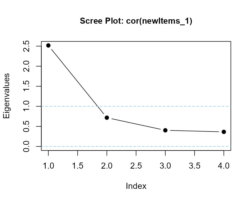(3)

#> cor(newItems_1)  is positive-definite
#> [1] 2.509 0.717 0.437 0.337

makeItemsScale() with same summated values and higher alpha

## apply makeItemsScale() function
newItems_2 <- makeItemsScale(
  scale = summatedScale,
  lowerbound = lowerbound,
  upperbound = upperbound,
  items = items,
  alpha = 0.9
)
#> generate 256 rows
#> rearrange 4 values within each of 256 rows
#> Complete!
#> desired Cronbach's alpha = 0.9 (achieved alpha = 0.8775)

### First 10 observations and summated scale
head(cbind(newItems_2, summatedScale), 10)
#>    V1 V2 V3 V4 summatedScale
#> 1   3  1  3  3            10
#> 2   4  2  4  4            14
#> 3   4  1  2  4            11
#> 4   4  1  1  2             8
#> 5   5  4  4  4            17
#> 6   3  2  2  2             9
#> 7   2  1  1  1             5
#> 8   4  2  2  2            10
#> 9   5  3  3  4            15
#> 10  3  1  2  3             9

### correlation matrix
cor(newItems_2) |> round(2)
#>      V1   V2   V3   V4
#> V1 1.00 0.59 0.61 0.68
#> V2 0.59 1.00 0.66 0.60
#> V3 0.61 0.66 1.00 0.70
#> V4 0.68 0.60 0.70 1.00

### requested Cronbach's alpha = 0.90
alpha(data = newItems_2) |> round(4)
#> [1] 0.8775

### calculate eigenvalues and print scree plot
eigenvalues(cor(newItems_2), 1) |> round(3)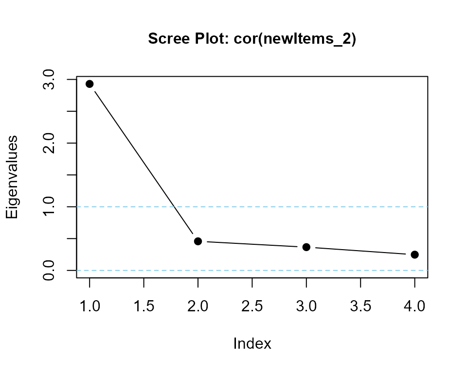

#> cor(newItems_2)  is positive-definite
#> [1] 2.926 0.436 0.370 0.268

same summated values with lower alpha may require higher variance

## apply makeItemsScale() function
newItems_3 <- makeItemsScale(
  scale = summatedScale,
  lowerbound = lowerbound,
  upperbound = upperbound,
  items = items,
  alpha = 0.6,
  variance = 0.7
)
#> generate 256 rows
#> rearrange 4 values within each of 256 rows
#> Complete!
#> desired Cronbach's alpha = 0.6 (achieved alpha = 0.6)

### First 10 observations and summated scale
head(cbind(newItems_3, summatedScale), 10)
#>    V1 V2 V3 V4 summatedScale
#> 1   3  1  3  3            10
#> 2   3  5  4  2            14
#> 3   2  5  2  2            11
#> 4   1  1  1  5             8
#> 5   3  4  5  5            17
#> 6   2  1  4  2             9
#> 7   1  1  2  1             5
#> 8   1  4  3  2            10
#> 9   2  4  4  5            15
#> 10  1  3  3  2             9

### correlation matrix
cor(newItems_3) |> round(2)
#>      V1   V2   V3   V4
#> V1 1.00 0.44 0.43 0.19
#> V2 0.44 1.00 0.28 0.13
#> V3 0.43 0.28 1.00 0.16
#> V4 0.19 0.13 0.16 1.00

### requested Cronbach's alpha = 0.70
alpha(data = newItems_3) |> round(4)
#> [1] 0.6

### calculate eigenvalues and print scree plot
eigenvalues(cor(newItems_3), 1) |> round(3)

#> cor(newItems_3)  is positive-definite
#> [1] 1.866 0.915 0.715 0.504

---

Create a dataframe for a t-test

Generating a data for an independent-samples t-test is trivial with LikertMakeR. But a dataframe for a paired-sample t-test is tricky because the observations are related to each other. That is, we must generate a dataframe of correlated observations.

Independent-samples t-test

Note that such tests don’t even require the same sample-size.

## define parameters
lower <- 1
upper <- 5
items <- 6

## generate two independent samples
x1 <- lfast(
  n = 20, mean = 2.5, sd = 0.75,
  lowerbound = lower, upperbound = upper, items = items
)
#> reached maximum of 1024 iterations
x2 <- lfast(
  n = 30, mean = 3.0, sd = 0.85,
  lowerbound = lower, upperbound = upper, items = items
)
#> reached maximum of 1024 iterations

## run independent-samples t-test
t.test(x1, x2)
#> 
#>  Welch Two Sample t-test
#> 
#> data:  x1 and x2
#> t = -2.186, df = 44.464, p-value = 0.03412
#> alternative hypothesis: true difference in means is not equal to 0
#> 95 percent confidence interval:
#>  -0.96083888 -0.03916112
#> sample estimates:
#> mean of x mean of y 
#>       2.5       3.0

makePaired() paired-sample t-test

makePaired() generates correlated values so the data replicate rating scales taken, for example, in a before and after experimental design. The function is effectively a wrapper function for lfast() and lcor() with the addition of a t-statistic from which the between-column correlation is inferred.

Paired t-tests apply to observations that are associated with each other. For example: the same people rating the same object before and after a treatment, the same people rating two different objects, ratings by husband & wife, etc.

makePaired() has similar parameters as for the lfast() function with the addition of a value for the desired t-statistic.

• n sample size

• means a [1:2] vector of target means for two before/after measures

• sds a [1:2] vector of target standard deviations

• t_value desired paired t-statistic

• lowerbound lower bound (e.g. ‘1’ for a 1-5 rating scale)

• upperbound upper bound (e.g. ‘5’ for a 1-5 rating scale)

• items number of items in the rating scale.

• precision can relax the level of accuracy required, as in lfast().

makePaired() examples

## define parameters
n <- 20
means <- c(2.5, 3.0)
sds <- c(0.75, 0.85)
lower <- 1
upper <- 5
items <- 6
t <- -2.5

## run the function
pairedDat <- makePaired(
  n = n, means = means, sds = sds,
  t_value = t,
  lowerbound = lower, upperbound = upper, items = items
)
#> Initial data vectors
#> best solution in 6 iterations
#> reached maximum of 1024 iterations
#> Arranging values to conform with desired t-value
#> Complete!

check properties of new data

## test function output
str(pairedDat)
#> 'data.frame':    20 obs. of  2 variables:
#>  $ X1: num  1.67 2.17 2.83 2.83 2.67 ...
#>  $ X2: num  1.33 3.17 3.5 2.33 1.83 ...

cor(pairedDat) |> round(2)
#>      X1   X2
#> X1 1.00 0.38
#> X2 0.38 1.00

pairedMoments <- data.frame(
  mean = apply(pairedDat, MARGIN = 2, FUN = mean) |> round(3),
  sd = apply(pairedDat, MARGIN = 2, FUN = sd) |> round(3)
) |> t()

pairedMoments
#>         X1    X2
#> mean 2.500 3.000
#> sd   0.749 0.845

run a paired-sample t-test with the new data

## run a paired-sample t-test

paired_t <- t.test(x = pairedDat$X1, y = pairedDat$X2, paired = TRUE)

# paired_t <- t.test(pairedDat$X1, pairedDat$X2, paired = TRUE)


paired_t
#> 
#>  Paired t-test
#> 
#> data:  pairedDat$X1 and pairedDat$X2
#> t = -2.5073, df = 19, p-value = 0.02141
#> alternative hypothesis: true mean difference is not equal to 0
#> 95 percent confidence interval:
#>  -0.91737903 -0.08262097
#> sample estimates:
#> mean difference 
#>            -0.5

---

Create a dataframe for Repeated-Measures ANOVA

makeRepeated()

makeRepeated() Reconstructs a synthetic dataset and inter-timepoint correlation matrix from a repeated-measures ANOVA result, based on reported means, standard deviations, and an F-statistic.

This function estimates the average correlation between repeated measures by matching the reported F-statistic, under one of three assumed correlation structures:

• "cs" (Compound Symmetry): Compound Symmetry assumes that all repeated measures are equally correlated with each other. That is, the correlation between time 1 and time 2 is the same as between time 1 and time 3, and so on. This structure is commonly used in repeated-measures ANOVA by default. It’s mathematically simple and reflects the idea that all timepoints are equally related. However, it may not be realistic for data where correlations decrease as time intervals increase (e.g., memory decay or learning effects).

• "ar1" (First-Order Autoregressive): first-order autoregressive, assumes that measurements closer together in time are more highly correlated than those further apart. For example, the correlation between time 1 and time 2 is stronger than between time 1 and time 3. This pattern is often realistic in longitudinal or time-series studies where change is gradual. The correlation drops off exponentially with each time step.

• "toeplitz" (Linearly Decreasing): Toeplitz structure is a more flexible option that allows the correlation between measurements to decrease linearly as the time gap increases. Unlike AR(1), where the decline is exponential, the Toeplitz structure assumes a straight-line drop in correlation.

makeRepeated() usage

makeRepeated(
  n, 
  k, 
  means, 
  sds,
  f_stat,
  df_between = k - 1,
  df_within = (n - 1) * (k - 1),
  structure = c("cs", "ar1", "toeplitz"),
  names = paste0("time_", 1:k),
  items = 1,
  lowerbound = 1, upperbound = 5,
  return_corr_only = FALSE,
  diagnostics = FALSE,
  ...
)

makeRepeated() arguments

• n Integer. Sample size used in the original study.
• k Integer. Number of repeated measures (timepoints).
• means Numeric vector of length k. Mean values reported for each timepoint.
• sds Numeric vector of length k. Standard deviations reported for each timepoint.
• f_stat Numeric. The reported repeated-measures ANOVA F-statistic for the within-subjects factor.
• df_between, Degrees of freedom between conditions (default: k - 1).
• df_within, Degrees of freedom within-subjects (default: (n - 1) * (k - 1)).
• structure Character. Correlation structure to assume: "cs", "ar1", or "toeplitz" (default).
• names Character vector of length k. Variable names for each timepoint (default: "time_1" to "time_k").
• items Integer. Number of items used to generate each scale score (passed to link{lfast}).
• lowerbound, Integer. Lower bounds for Likert-type response scales (default: 1).
• upperbound, Integer. upper bounds for Likert-type response scales (default: 5).
• return_corr_only Logical. If TRUE, return only the estimated correlation matrix.
• diagnostics Logical. If TRUE, include diagnostic summaries such as feasible F-statistic range and effect sizes.

makeRepeated() examples

out1 <- makeRepeated(
  n = 128,
  k = 3,
  means = c(3.1, 3.5, 3.9),
  sds = c(1.0, 1.1, 1.0),
  items = 4,
  f_stat = 4.87,
  structure = "cs",
  diagnostics = FALSE
)
#> Warning in makeRepeated(n = 128, k = 3, means = c(3.1, 3.5, 3.9), sds = c(1, :
#> Optimization may not have converged. Check results carefully.
#> best solution in 413 iterations
#> best solution in 1112 iterations
#> best solution in 758 iterations

head(out1$data)
#>   time_1 time_2 time_3
#> 1   3.75   4.50   2.25
#> 2   1.50   5.00   4.00
#> 3   3.00   2.25   5.00
#> 4   3.75   3.00   3.75
#> 5   1.25   4.75   4.50
#> 6   4.25   4.75   1.25
out1$correlation_matrix
#>            time_1     time_2     time_3
#> time_1  1.0000000 -0.4899454 -0.4899454
#> time_2 -0.4899454  1.0000000 -0.4899454
#> time_3 -0.4899454 -0.4899454  1.0000000


out2 <- makeRepeated(
  n = 32, k = 4,
  means = c(2.75, 3.5, 4.0, 4.4),
  sds = c(0.8, 1.0, 1.2, 1.0),
  f_stat = 16,
  structure = "ar1",
  items = 5,
  lowerbound = 1, upperbound = 7,
  return_corr_only = FALSE,
  diagnostics = TRUE
)
#> reached maximum of 1024 iterations
#> reached maximum of 1024 iterations
#> reached maximum of 1024 iterations
#> reached maximum of 1024 iterations

print(out2)
#> $data
#>    time_1 time_2 time_3 time_4
#> 1     2.2    3.6    4.4    5.0
#> 2     4.2    4.6    4.2    3.6
#> 3     3.6    4.0    3.6    3.6
#> 4     2.8    5.8    5.8    6.0
#> 5     3.4    4.4    6.4    4.4
#> 6     4.6    4.6    2.2    4.4
#> 7     2.8    5.0    4.4    4.0
#> 8     2.8    3.4    4.0    5.6
#> 9     2.0    3.6    4.6    5.8
#> 10    3.0    3.0    3.2    4.0
#> 11    1.8    2.6    2.6    4.6
#> 12    1.6    1.6    3.4    4.4
#> 13    4.0    2.6    4.6    5.0
#> 14    2.4    2.4    3.2    4.4
#> 15    3.0    4.0    2.6    4.2
#> 16    3.4    4.6    4.6    4.4
#> 17    1.8    2.0    4.4    4.0
#> 18    2.8    2.2    4.0    3.0
#> 19    2.8    3.6    2.8    1.8
#> 20    2.2    3.6    5.6    4.0
#> 21    3.0    3.0    5.4    5.2
#> 22    3.0    3.4    6.0    5.0
#> 23    2.4    2.8    3.0    6.0
#> 24    2.2    2.6    2.2    3.4
#> 25    3.6    4.2    5.2    4.4
#> 26    2.0    3.8    3.8    3.4
#> 27    1.6    5.0    3.6    3.6
#> 28    3.6    3.0    2.8    5.0
#> 29    1.4    2.8    3.2    3.8
#> 30    3.0    3.4    4.8    4.0
#> 31    2.8    4.6    5.6    6.8
#> 32    2.2    2.2    2.0    3.8
#> 
#> $correlation_matrix
#>            time_1    time_2    time_3     time_4
#> time_1 1.00000000 0.3910032 0.1528835 0.05977794
#> time_2 0.39100319 1.0000000 0.3910032 0.15288350
#> time_3 0.15288350 0.3910032 1.0000000 0.39100319
#> time_4 0.05977794 0.1528835 0.3910032 1.00000000
#> 
#> $structure
#> [1] "ar1"
#> 
#> $feasible_f_range
#>       min       max 
#>  9.353034 39.481390 
#> 
#> $recommended_f
#> $recommended_f$conservative
#> [1] 10.21
#> 
#> $recommended_f$moderate
#> [1] 11.91
#> 
#> $recommended_f$strong
#> [1] 30.29
#> 
#> 
#> $achieved_f
#> [1] 15.99983
#> 
#> $effect_size_raw
#> [1] 0.3792188
#> 
#> $effect_size_standardised
#> [1] 0.3717831


out3 <- makeRepeated(
  n = 32, k = 4,
  means = c(2.0, 2.5, 3.0, 2.8),
  sds = c(0.8, 0.9, 1.0, 0.9),
  items = 4,
  f_stat = 24,
  structure = "toeplitz",
  diagnostics = TRUE
)
#> Warning in makeRepeated(n = 32, k = 4, means = c(2, 2.5, 3, 2.8), sds = c(0.8,
#> : Optimization may not have converged. Check results carefully.
#> best solution in 683 iterations
#> reached maximum of 1024 iterations
#> reached maximum of 1024 iterations
#> reached maximum of 1024 iterations

str(out3)
#> List of 8
#>  $ data                    :'data.frame':    32 obs. of  4 variables:
#>   ..$ time_1: num [1:32] 1 1.25 2.75 1.25 3 4 1.75 3 2.5 2 ...
#>   ..$ time_2: num [1:32] 1.25 2 3 1.25 2.25 3.5 4 2.75 2.75 1.5 ...
#>   ..$ time_3: num [1:32] 3.25 2.25 3.25 1.25 3.5 2 4.5 3 4.5 3.5 ...
#>   ..$ time_4: num [1:32] 2.5 2.25 2.25 1.5 2.5 1.25 4 1.5 4.75 3.5 ...
#>  $ correlation_matrix      : num [1:4, 1:4] 1 0.66 0.33 0 0.66 ...
#>   ..- attr(*, "dimnames")=List of 2
#>   .. ..$ : chr [1:4] "time_1" "time_2" "time_3" "time_4"
#>   .. ..$ : chr [1:4] "time_1" "time_2" "time_3" "time_4"
#>  $ structure               : chr "toeplitz"
#>  $ feasible_f_range        : Named num [1:2] 5.57 8.64
#>   ..- attr(*, "names")= chr [1:2] "min" "max"
#>  $ recommended_f           :List of 3
#>   ..$ conservative: num 5.59
#>   ..$ moderate    : num 5.62
#>   ..$ strong      : num 7.64
#>  $ achieved_f              : num 9.95
#>  $ effect_size_raw         : num 0.142
#>  $ effect_size_standardised: num 0.174

---

Generate rating-scale data from multiple regression results

makeScalesRegression()

Generates synthetic rating-scale data that replicates reported regression results: standardised betas, R^2, and correlation matrix of independent variables (if available).

makeScalesRegression() usage

makeScalesRegression <- (
   n, 
   beta_std, 
   r_squared, 
   iv_cormatrix = NULL, 
   iv_cor_mean = 0.3,  
   iv_cor_variance = 0.01, 
   iv_cor_range = c(-0.7, 0.7), 
   iv_means, 
   iv_sds,  
   dv_mean,  
   dv_sd, 
   lowerbound_iv,  
   upperbound_iv,  
   lowerbound_dv, 
   upperbound_dv,  
   items_iv = 1,  
   items_dv = 1,  
   var_names = NULL,  
   tolerance = 0.005 
)

makeScalesRegression() arguments

• n sample size.
• beta_std a vector of length k (number of independent variables) of standardised betas.
• r_squared model R^2
• iv_cormatrix independent variables correlation matrix. Default= NULL
• iv_cor_mean if no iv_cormatrix, average IV correlations. Default = 0.3
• iv_cor_variance if no iv_cormatrix, variation in iv_cormatrix. Default = 0.01
• iv_cor_range if no iv_cormatrix, range in iv_cormatrix. Default = c(-0.7, 0.7)
• iv_means a vector of length k of IV mean values
• iv_sds a vector of length k of IV standard deviations
• dv_mean mean of Dependent Variable (DV)
• dv_sd standard deviation of DV
• lowerbound_iv a vector of length k of lowerbounds for IV’s
• upperbound_iv a vector of length k of upperbounds for IV’s
• lowerbound_dv lowerbound for DV
• upperbound_dv upperbound for DV
• items_iv a vector of length k of number of items in the IV’s. Default = 1.
• items_dv number of items in DV. Default = 1.
• var_names a vector of variable names (Independent Variables first then the Dependent Variable). Default = NULL
• tolerance close to target R-squared. Default = 0.005

makeScalesRegression() examples

Example 1: With provided IV correlation matrix

set.seed(123)
iv_corr <- matrix(c(1.0, 0.3, 0.3, 1.0), nrow = 2)

result1 <- makeScalesRegression(
  n = 64,
  beta_std = c(0.4, 0.3),
  r_squared = 0.35,
  iv_cormatrix = iv_corr,
  iv_means = c(3.0, 3.5),
  iv_sds = c(1.0, 0.9),
  dv_mean = 3.8,
  dv_sd = 1.1,
  lowerbound_iv = 1,
  upperbound_iv = 5,
  lowerbound_dv = 1,
  upperbound_dv = 5,
  items_iv = 4,
  items_dv = 4,
  var_names = c("Attitude", "Intention", "Behaviour")
)

print(result1)
head(result1$data)

Example 2: With optimisation (no IV correlation matrix)

set.seed(456)
result2 <- makeScalesRegression(
  n = 64,
  beta_std = c(0.3, 0.25, 0.2),
  r_squared = 0.40,
  iv_cormatrix = NULL, # Will be optimised
  iv_cor_mean = 0.3,
  iv_cor_variance = 0.02,
  iv_means = c(3.0, 3.2, 2.8),
  iv_sds = c(1.0, 0.9, 1.1),
  dv_mean = 3.5,
  dv_sd = 1.0,
  lowerbound_iv = 1,
  upperbound_iv = 5,
  lowerbound_dv = 1,
  upperbound_dv = 5,
  items_iv = 4,
  items_dv = 5
)

# View optimised correlation matrix
print(result2$target_stats$iv_cormatrix)
print(result2$optimisation_info)

---

Create a multidimensional dataframe of correlated scale items

correlateScales()

Correlated rating-scale items generally are summed or averaged to create a measure of an “unobservable”, or “latent”, construct.

correlateScales() takes several such dataframes of rating-scale items and rearranges their rows so that the scales are correlated according to a predefined correlation matrix. Univariate statistics for each dataframe of rating-scale items do not change, but their correlations with rating-scale items in other dataframes do.

To run correlateScales(), parameters are:

• dataframes: a list of ‘k’ dataframes to be rearranged and combined

• scalecors: target correlation matrix - should be a symmetric k*k positive-semi-definite matrix, where ‘k’ is the number of dataframes

As with other functions in LikertMakeR, correlateScales() focuses on item and scale moments (mean and standard deviation) rather than on covariance structure. If you wish to simulate data for teaching or experimenting with Structural Equation modelling, then I recommend the sim.item() and sim.congeneric() functions from the psych package

correlateScales() examples

three attitudes and a behavioural intention

create dataframes of Likert-scale items

n <- 128
lower <- 1
upper <- 5

### attitude #1

#### generate a correlation matrix
cor_1 <- makeCorrAlpha(items = 4, alpha = 0.80)
#> reached max iterations (1600) - best mean difference: 4.6e-05

#### specify moments as vectors
means_1 <- c(2.5, 2.5, 3.0, 3.5)
sds_1 <- c(0.75, 0.85, 0.85, 0.75)

#### apply makeItems() function
Att_1 <- makeItems(
  n = n, means = means_1, sds = sds_1,
  lowerbound = rep(lower, 4), upperbound = rep(upper, 4),
  cormatrix = cor_1
)
#> NOTE:
#> makeItems() function is being deprecated
#>               
#> Use the makeScales() function in future.
#> Variable  1
#> reached maximum of 16384 iterations
#> Variable  2
#> best solution in 1475 iterations
#> Variable  3
#> best solution in 171 iterations
#> Variable  4
#> reached maximum of 16384 iterations
#> 
#> Arranging data to match correlations
#> 
#> Successfully generated correlated variables

### attitude #2

#### generate a correlation matrix
cor_2 <- makeCorrAlpha(items = 5, alpha = 0.85)
#> reached max iterations (2500) - best mean difference: 4e-05

#### specify moments as vectors
means_2 <- c(2.5, 2.5, 3.0, 3.0, 3.5)
sds_2 <- c(0.75, 0.85, 0.75, 0.85, 0.75)

#### apply makeItems() function
Att_2 <- makeItems(
  n, means_2, sds_2,
  rep(lower, 5), rep(upper, 5),
  cor_2
)
#> NOTE:
#> makeItems() function is being deprecated
#>               
#> Use the makeScales() function in future.
#> Variable  1
#> reached maximum of 16384 iterations
#> Variable  2
#> best solution in 34 iterations
#> Variable  3
#> reached maximum of 16384 iterations
#> Variable  4
#> best solution in 234 iterations
#> Variable  5
#> reached maximum of 16384 iterations
#> 
#> Arranging data to match correlations
#> 
#> Successfully generated correlated variables

### attitude #3

#### generate a correlation matrix
cor_3 <- makeCorrAlpha(items = 6, alpha = 0.90)
#> reached max iterations (3600) - best mean difference: 4e-05
#> Correlation matrix is not yet positive definite
#> Working on it
#> 
#> improved at swap - 2 (min eigenvalue: -0.031507)
#> improved at swap - 6 (min eigenvalue: -0.018702)
#> improved at swap - 7 (min eigenvalue: -0.010675)
#> improved at swap - 10 (min eigenvalue: 0.052317)
#> positive definite at swap - 10

#### specify moments as vectors
means_3 <- c(2.5, 2.5, 3.0, 3.0, 3.5, 3.5)
sds_3 <- c(0.75, 0.85, 0.85, 1.0, 0.75, 0.85)

#### apply makeItems() function
Att_3 <- makeItems(
  n, means_3, sds_3,
  rep(lower, 6), rep(upper, 6),
  cor_3
)
#> NOTE:
#> makeItems() function is being deprecated
#>               
#> Use the makeScales() function in future.
#> Variable  1
#> reached maximum of 16384 iterations
#> Variable  2
#> best solution in 1140 iterations
#> Variable  3
#> best solution in 41 iterations
#> Variable  4
#> reached maximum of 16384 iterations
#> Variable  5
#> reached maximum of 16384 iterations
#> Variable  6
#> best solution in 561 iterations
#> 
#> Arranging data to match correlations
#> 
#> Successfully generated correlated variables

### behavioural intention
intent <- lfast(n, mean = 4.0, sd = 3, lowerbound = 0, upperbound = 10) |>
  data.frame()
#> best solution in 1305 iterations
names(intent) <- "int"

check properties of item dataframes

## Attitude #1
A1_moments <- data.frame(
  means = apply(Att_1, 2, mean) |> round(2),
  sds = apply(Att_1, 2, sd) |> round(2)
) |> t()

### Attitude #1 moments
A1_moments
#>       item01 item02 item03 item04
#> means   2.50   2.50   3.00   3.50
#> sds     0.75   0.85   0.85   0.75

### Attitude #1 correlations
cor(Att_1) |> round(2)
#>        item01 item02 item03 item04
#> item01   1.00   0.49   0.37   0.51
#> item02   0.49   1.00   0.65   0.68
#> item03   0.37   0.65   1.00   0.28
#> item04   0.51   0.68   0.28   1.00

### Attitude #1 cronbach's alpha
alpha(cor(Att_1)) |> round(3)
#> [1] 0.798

## Attitude #2
A2_moments <- data.frame(
  means = apply(Att_2, 2, mean) |> round(2),
  sds = apply(Att_2, 2, sd) |> round(2)
) |> t()

### Attitude #2 moments
A2_moments
#>       item01 item02 item03 item04 item05
#> means   2.50   2.50   3.00   3.00   3.50
#> sds     0.75   0.85   0.75   0.85   0.75

### Attitude #2 correlations
cor(Att_2) |> round(2)
#>        item01 item02 item03 item04 item05
#> item01   1.00   0.61   0.54   0.74   0.61
#> item02   0.61   1.00   0.41   0.47   0.44
#> item03   0.54   0.41   1.00   0.60   0.35
#> item04   0.74   0.47   0.60   1.00   0.53
#> item05   0.61   0.44   0.35   0.53   1.00

### Attitude #2 cronbach's alpha
alpha(cor(Att_2)) |> round(3)
#> [1] 0.849

## Attitude #3
A3_moments <- data.frame(
  means = apply(Att_3, 2, mean) |> round(2),
  sds = apply(Att_3, 2, sd) |> round(2)
) |> t()

### Attitude #3 moments
A3_moments
#>       item01 item02 item03 item04 item05 item06
#> means   2.50   2.50   3.00      3   3.50   3.50
#> sds     0.75   0.85   0.85      1   0.75   0.85

### Attitude #3 correlations
cor(Att_3) |> round(2)
#>        item01 item02 item03 item04 item05 item06
#> item01   1.00   0.52   0.79   0.43   0.71   0.63
#> item02   0.52   1.00   0.71   0.86   0.47   0.41
#> item03   0.79   0.71   1.00   0.70   0.71   0.65
#> item04   0.43   0.86   0.70   1.00   0.43   0.46
#> item05   0.71   0.47   0.71   0.43   1.00   0.42
#> item06   0.63   0.41   0.65   0.46   0.42   1.00

### Attitude #2 cronbach's alpha
alpha(cor(Att_3)) |> round(3)
#> [1] 0.897


## Behavioural Intention

intent_moments <- data.frame(
  mean = apply(intent, 2, mean) |> round(3),
  sd = apply(intent, 2, sd) |> round(3)
) |> t()

### Intention moments
intent_moments
#>        int
#> mean 4.000
#> sd   2.999

correlateScales parameters

### target scale correlation matrix
scale_cors <- matrix(
  c(
    1.0, 0.7, 0.6, 0.5,
    0.7, 1.0, 0.4, 0.3,
    0.6, 0.4, 1.0, 0.2,
    0.5, 0.3, 0.2, 1.0
  ),
  nrow = 4
)

### bring dataframes into a list
data_frames <- list("A1" = Att_1, "A2" = Att_2, "A3" = Att_3, "Int" = intent)

apply the correlateScales() function

### apply correlateScales() function
my_correlated_scales <- correlateScales(
  dataframes = data_frames,
  scalecors = scale_cors
)
#> scalecors  is positive-definite
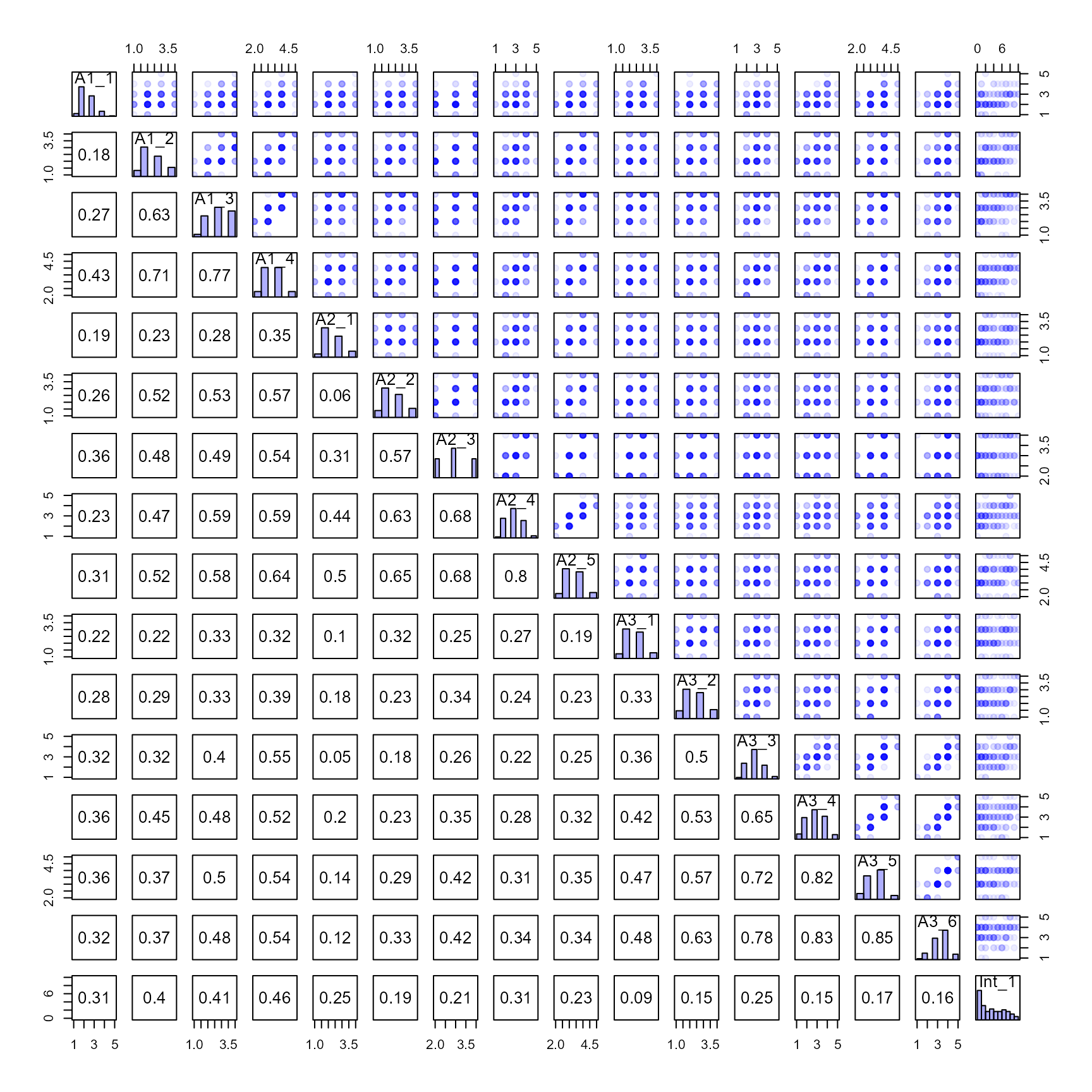
#> New dataframe successfully created

plot the new correlated scale items

Check the properties of our derived dataframe

## data structure
str(my_correlated_scales)
#> 'data.frame':    128 obs. of  16 variables:
#>  $ A1_1 : num  2 3 2 3 2 3 4 2 2 2 ...
#>  $ A1_2 : num  2 3 1 2 2 4 3 1 2 1 ...
#>  $ A1_3 : num  3 3 2 2 3 4 3 2 2 3 ...
#>  $ A1_4 : num  3 4 3 4 3 4 4 3 3 2 ...
#>  $ A2_1 : num  2 3 2 3 2 4 3 1 2 1 ...
#>  $ A2_2 : num  2 2 3 4 3 4 4 1 2 2 ...
#>  $ A2_3 : num  3 3 2 4 3 4 3 3 3 2 ...
#>  $ A2_4 : num  1 3 2 3 3 4 3 2 3 2 ...
#>  $ A2_5 : num  3 4 3 4 4 4 4 2 4 3 ...
#>  $ A3_1 : num  1 3 2 3 2 2 3 3 2 2 ...
#>  $ A3_2 : num  2 3 2 3 3 1 2 2 2 2 ...
#>  $ A3_3 : num  2 4 2 3 3 2 4 3 2 2 ...
#>  $ A3_4 : num  2 4 2 3 4 2 3 2 2 2 ...
#>  $ A3_5 : num  3 3 2 4 3 3 4 4 2 3 ...
#>  $ A3_6 : num  2 4 3 3 3 4 4 3 4 3 ...
#>  $ Int_1: num  4 3 1 4 2 2 6 7 0 0 ...

## eigenvalues of dataframe correlations
Cor_Correlated_Scales <- cor(my_correlated_scales)
eigenvalues(cormatrix = Cor_Correlated_Scales, scree = TRUE) |> round(2)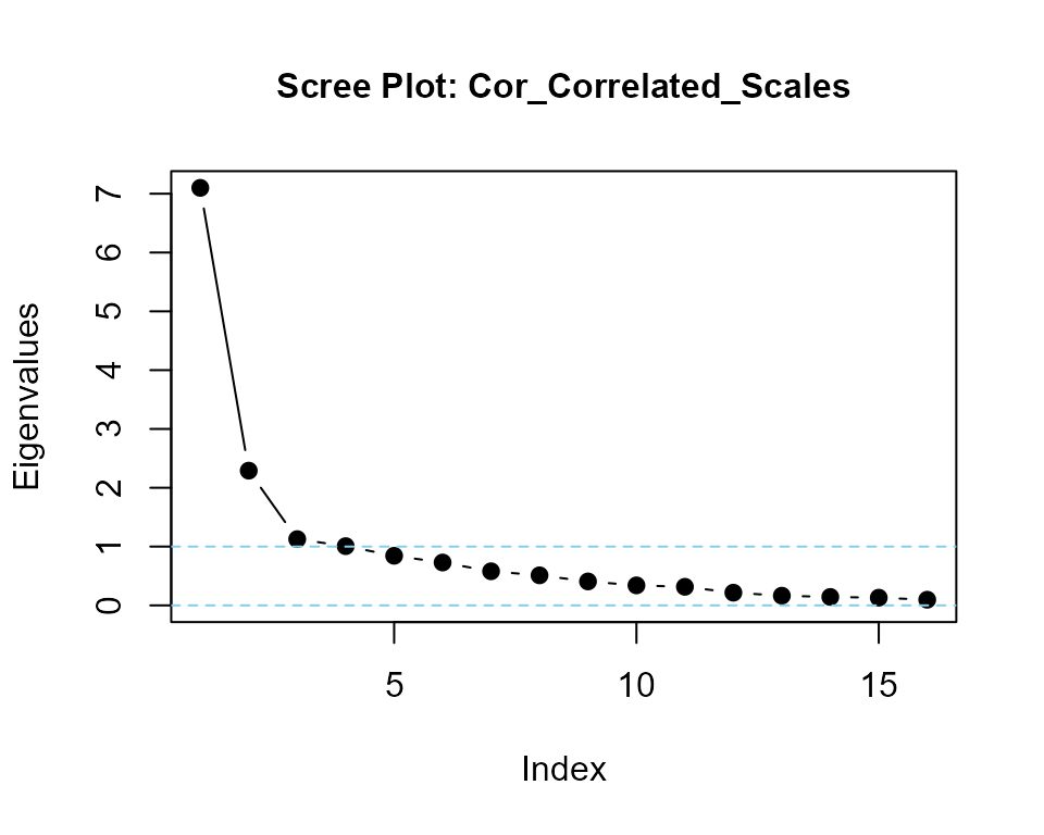

#> Cor_Correlated_Scales  is positive-definite
#>  [1] 6.92 2.26 1.13 0.98 0.78 0.66 0.57 0.56 0.52 0.43 0.32 0.29 0.19 0.16 0.14
#> [16] 0.10

#### Eigenvalues of predictor variable items only
Cor_Attitude_items <- cor(my_correlated_scales[, -16])
eigenvalues(cormatrix = Cor_Attitude_items, scree = TRUE) |> round(2)

#> Cor_Attitude_items  is positive-definite
#>  [1] 6.76 2.23 1.00 0.86 0.69 0.65 0.56 0.54 0.49 0.34 0.29 0.19 0.16 0.14 0.10

---

Helper functions

likertMakeR() includes two additional functions that may be of help when examining parameters and output.

• alpha() calculates Cronbach’s Alpha from a given correlation matrix or a given dataframe

• eigenvalues() calculates eigenvalues of a correlation matrix, a report on whether the correlation matrix is positive definite, and produces an optional scree plot.

alpha()

alpha() accepts, as input, either a correlation matrix or a dataframe. If both are submitted, then the correlation matrix is used by default, with a message to that effect.

alpha() examples

## define parameters
df <- data.frame(
  V1 = c(4, 2, 4, 3, 2, 2, 2, 1),
  V2 = c(3, 1, 3, 4, 4, 3, 2, 3),
  V3 = c(4, 1, 3, 5, 4, 1, 4, 2),
  V4 = c(4, 3, 4, 5, 3, 3, 3, 3)
)

corMat <- matrix(
  c(
    1.00, 0.35, 0.45, 0.75,
    0.35, 1.00, 0.65, 0.55,
    0.45, 0.65, 1.00, 0.65,
    0.75, 0.55, 0.65, 1.00
  ),
  nrow = 4, ncol = 4
)

## apply function examples
alpha(cormatrix = corMat)
#> [1] 0.8395062
alpha(data = df)
#> [1] 0.8026658
alpha(NULL, df)
#> [1] 0.8026658
alpha(corMat, df)
#> Alert: 
#> Both cormatrix and data present.
#>                 
#> Using cormatrix by default.
#> [1] 0.8395062

eigenvalues()

eigenvalues() calculates eigenvalues of a correlation matrix, reports on whether the matrix is positive-definite, and optionally produces a scree plot.

eigenvalues() examples

## define parameters
correlationMatrix <- matrix(
  c(
    1.00, 0.25, 0.35, 0.45,
    0.25, 1.00, 0.70, 0.75,
    0.35, 0.70, 1.00, 0.85,
    0.45, 0.75, 0.85, 1.00
  ),
  nrow = 4, ncol = 4
)

## apply function
evals <- eigenvalues(cormatrix = correlationMatrix)
#> correlationMatrix  is positive-definite

print(evals)
#> [1] 2.7484991 0.8122627 0.3048151 0.1344231

eigenvalues() function with optional scree plot

evals <- eigenvalues(correlationMatrix, 1)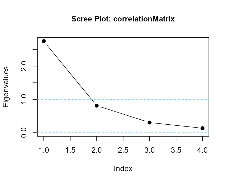

#> correlationMatrix  is positive-definite
print(evals)
#> [1] 2.7484991 0.8122627 0.3048151 0.1344231

---

Alternative methods & packages

LikertMakeR is intended for synthesising & correlating rating-scale data with means, standard deviations, and correlations as close as possible to predefined parameters. If you don’t need your data to be close to exact, then other options may be faster or more flexible.

Different approaches include:

• sampling from a truncated normal distribution

• sampling with a predetermined probability distribution

• marginal model specification

sampling from a truncated normal distribution

Data are sampled from a normal distribution, and then truncated to suit the rating-scale boundaries, and rounded to set discrete values as we see in rating scales.

See Heinz (2021) for an excellent and short example using the following packages:

• truncnorm

• faux

• See also the rLikert() function from the excellent latent2likert package, Lalovic (2024), for an approach using optimal discretization and skew-normal distribution. latent2likert() converts continuous latent variables into ordinal categories to generate Likert scale item responses.

sampling with a predetermined probability distribution

• the following code will generate a vector of values with approximately the given probabilities. Good for simulating a single item.

n <- 128
sample(1:5, n,
  replace = TRUE,
  prob = c(0.1, 0.2, 0.4, 0.2, 0.1)
)

marginal model specification

Marginal model specification extends the idea of a predefined probability distribution to multivariate and correlated dataframes.

• SimCorrMix: Simulation of Correlated Data with Multiple Variable Types Including Continuous and Count Mixture Distributions on CRAN.

• SimMultiCorrData: Simulation of Correlated Data with Multiple Variable Types on CRAN.

• lsasim: Functions to Facilitate the Simulation of Large Scale Assessment Data on CRAN. See Matta et al. (2018)

• GenOrd:Simulation of Discrete Random Variables with Given Correlation Matrix and Marginal Distributions on CRAN.

• SimCorMultRes: Simulates Correlated Multinomial Responses on CRAN. See Touloumis (2016)

• covsim: VITA, IG and PLSIM Simulation for Given Covariance and Marginals on CRAN. See Grønneberg et al. (2022)

Factor Models: Classical Test Theory (CTT)

The psych package has several excellent functions for simulating rating-scale data based on factor loadings.
These focus on factor and item correlations rather than item moments.
Highly recommended.

• psych::sim.item Generate simulated data structures for circumplex, spherical, or simple structure

• psych::sim.congeneric Simulate a congeneric data set with or without minor factors See Revelle (in prep)

Also:

simsem has many functions for simulating and testing data for application in Structural Equation modelling. See examples at https://simsem.org/

General data simulation

simpr provides a general, simple, and tidyverse-friendly framework for generating simulated data, fitting models on simulations, and tidying model results.

---

References

D’Alessandro, S., H. Winzar, B. Lowe, B.J. Babin, W. Zikmund (2020). Marketing Research 5^ed, Cengage Australia. https://cengage.com.au/sem121/marketing-research-5th-edition-dalessandro-babin-zikmund

Grønneberg, S., Foldnes, N., & Marcoulides, K. M. (2022). covsim: An R Package for Simulating Non-Normal Data for Structural Equation Models Using Copulas. Journal of Statistical Software, 102(1), 1–45. doi:10.18637/jss.v102.i03

Heinz, A. (2021), Simulating Correlated Likert-Scale Data In R: 3 Simple Steps (blog post) https://glaswasser.github.io/simulating-correlated-likert-scale-data/

Lalovic M (2024). latent2likert: Converting Latent Variables into Likert Scale Responses. R package version 1.2.2, https://latent2likert.lalovic.io/.

Matta, T.H., Rutkowski, L., Rutkowski, D. & Liaw, Y.L. (2018), lsasim: an R package for simulating large-scale assessment data. Large-scale Assessments in Education 6, 15. doi:10.1186/s40536-018-0068-8

Pornprasertmanit, S., Miller, P., & Schoemann, A. (2021). simsem: R package for simulated structural equation modeling https://simsem.org/

Revelle, W. (in prep) An introduction to psychometric theory with applications in R. Springer. (working draft available at https://personality-project.org/r/book/ )

Touloumis, A. (2016), Simulating Correlated Binary and Multinomial Responses under Marginal Model Specification: The SimCorMultRes Package, The R Journal 8:2, 79-91. doi:10.32614/RJ-2016-034

Winzar, H. (2022). LikertMakeR: Synthesise and correlate Likert scale and related rating-scale data with predefined first and second moments. CRAN: doi:10.32614/CRAN.package.LikertMakeR