LikertMakeR Scale Reproduction Validation
Hume Winzar
September 2025
Source:vignettes/lfast_validation.Rmd
lfast_validation.RmdLikertMakeR Validation
This paper reports on a study that compares data produced using LikertMakeR with original data from a published and publicly-available source.
Abstract
The LikertMakeR::lfast() function generally produces
surprisingly good replications of existing data.
Data distributions usually are unimodal, so multimodal (or wiggly) data are poorly represented.
Highly leptokurtic data (pointy with wide tails) also may be poorly represented.
These exceptions are likely to occur when more than one utility function is included in the original sample data. That is, when different groups of respondents are joined together.
Validation against real data
One objective of the LikertMakeR package (winzar2022?) is to “reproduce” or “reverse engineer” rating-scale data for further analysis and visualization when only summary statistics are available. In such a role, the synthetic data should accurately represent the original data, meaning both should plausibly originate from the same population.
To validate synthetic data, we choose a data set that is readily available, and which can be filtered to represent rating-scale data that may be commonly seen in published reports.
We should compare data with variations in:
- sample sizes,
- number of increments in a scale. Number of increments may be defined
by:
- number of items in the scale
- length of the scale item (1 to 5; 0 to 10; etc.)
- modality: the extent that a distribution shows bumps or something other than a smooth hill.
SPI (SAPA Personality Inventory)
For convenience and reproducibility, I chose a subsample of the SAPA Personality Inventory (Condon 2023) data available from the psych (Revelle 2024) and psychtools (William Revelle 2024) packages for R. The data set holds 4000 observations of 145 variables.
Variable/ scale selection
The SPI is based on a hierarchical framework for assessing personality at two levels. The higher level has the familiar “Big Five” factors that have been studied in personality research since the 1980s.
In the SPI, each of these five dimensions is represented by
the average of fourteen 6-point agree-disagree items. That is,
scale values have a scale with 14 * 6 = 84 possible
values.
| Big Five Personality Dimensions |
|---|
| Conscientiousness |
| Agreeableness |
| Neuroticism |
| Openness |
| Extraversion |
The lower level has 27 factors, made by averaging five
6-point items, most of which are sub-scales of the Big Five. These give
scales with 5 * 6 = 30 possible values.
| Adaptability | Anxiety | ArtAppreciation |
| AttentionSeeking | Authoritarianism | Charisma |
| Compassion | Conformity | Conservatism |
| Creativity | EasyGoingness | EmotionalExpressiveness |
| EmotionalStability | Honesty | Humor |
| Impulsivity | Industry | Intellect |
| Introspection | Irritability | Order |
| Perfectionism | SelfControl | SensationSeeking |
| Sociability | Trust | WellBeing |
Finally, these dimensions and facets are made by averaging subsets of
135 items (individual questions). Each item then is a scale with
1 * 6 = 6 possible values.
| Property | Dimensions | Facets | Items |
|---|---|---|---|
| Number of scales | 5 | 27 | 135 |
| Items per scale | 14 | 5 | 1 |
| Discrete values per scale | 84 | 30 | 6 |
Measures of Difference
The function LikertMakeR::lfast() produces a vector of
values with predefined first and second moments usually correct to two
decimal places. Vectors also have exact minima & maxima, and scale
intervals.
To determine whether synthetic data are no different from the data that produced the original summary statistics, we need something more than just equal mean and standard deviation. We need measures that can accommodate third and fourth moments (skewness and kurtosis) as well. Further, a comparison should accommodate occasional bimodal distributions that may occur.
Choice of Test for Equal Distributions
To assess the similarity between synthetic data generated by LikertMakeR and real survey data, we evaluate the agreement between their empirical distributions using nonparametric two-sample tests.
Several tests are available for comparing continuous distributions:
The Kolmogorov–Smirnov (KS) test focuses on the maximum vertical distance between the empirical cumulative distribution functions (ECDFs) of the two samples. The KS test has reduced sensitivity near the centre of the distribution and excessive sensitivity to extreme values (Lilliefors 1967).
The Baumgartner–Weiß–Schindler (BWS) test (Baumgartner et al. 1998)
improves upon the KS test by incorporating differences across the entire distribution, using a rank-based test statistic derived from integrated spacing differences. The BWS test is more powerful than either the Kolmogorov-Smirnov test or the Wilcoxon test (Pav 2023), as shown in Baumgartner et al. (1998). It is sensitive to both location and shape differences and generally has greater power across a variety of alternatives (Neuhäuser 2001; Neuhäuser and Ruxton 2009).The Neuhäuser modification of the BWS test introduces a weighting function that emphasizes differences in the central region of the distribution while reducing the influence of the tails (Neuhäuser 2001). This makes it more robust to small discrepancies in the extremes — a desirable property in large samples where minor tail mismatches can lead to false positives (Neuhäuser 2005).
Overall, The researcher might want to use the BWS test to
see if LikertMakeR::lfast() gives an exact
replication of a scale, and use the Neuhäuser test option
to see if the function produces a “pretty good” dataframe. So, we
present summary results for both tests in this study.
| Feature | method = “BWS” | method = “Neuhäuser” |
|---|---|---|
| Test Statistic | Based on comparing quantiles | Based on comparing ranks. |
| Sensitivity | More sensitive to shape differences. | Less sensitive to shape differences. |
| Robustness to Outliers | Less robust to outliers. | More robust to outliers. |
| Focus | Sensitive to general differences across the ranks | Less sensitive to tail differences. |
| Type of Differences | More likely to pick up on subtle differences | Less likely to pick up on subtle differences |
Research Design
We suspect that the accuracy of data created by
LikertMakeR::lfast() will be affected by:
- the shape of the true distribution
- sample-size
- number of discrete intervals in a scale
That is, highly skewed and multimodal distributions, and smaller
sample sizes, are likely to be less well replicated by synthetic data
generated by LikertMakeR::lfast().
Data selection
The SPI dataset includes demographic information on which we can filter the 4000 observations down to sample-sizes that we are more likely to find in normal social research. Somewhat arbitrarily, I decided to use Age, Gender, and Education as filters.
Small sample
Young highly-educated men
young_highly_educated_men <- spi |>
  filter(age < 24 & sex == 1 & education == 7)

## where, sex==1 = 'male'
##        education == 7 = 'postgraduate degree'
This filtering produced a sample of 19 observations.
Medium sample
Young educated women
young_educated_women <- spi |>
  filter(age < 24 & sex == 2 & education >= 5)

## where, "sex==2" = 'female'
##        "education >= 5" = 'undergraduate degree or higher'
This filtering produced a sample of 99 observations.
Large sample
Young school-leavers
under_18_highschool <- spi |>
  filter(age < 18 & education == 1)

## where, "education == 1" = 'Less than 12 years schooling'
This filtering produced a sample of 314 observations.
Procedure
We have three samples with small, medium and large sample-sizes.
- small, 19 observations
- medium, 99 observations
- large, 314 observations
And we have three levels of data aggregation:
- 5 dimensions, each of 14 items
- 27 factors, each of 5 items
- 135 individual items
This gives us (3 * (5 + 27 + 135) = 501) data
subsets.
For each combination of sample and data-level we find the mean and
standard deviation of the data subset, then apply the
LikertMakeR::lfast function to produce
2^10 = 1024 simulated dataframes to compare with the true
original dataframes from the SPI data.
We compare the Empirical Cumulative Density Function (ECDF) of each simulated dataframe with the ECDF of the original dataframe using both the BWS and Neuhäuser methods. With more than 1000 tests on each of 501 original dataframes we should be able to see how accurate our simulations are.
Original Data
We present charts as summary information about the three levels of data under consideration. These are bar-charts for each measurement level combined with kernel density estimates.
SPI Big Five Dimensions
Each of the Big Five measures is the average of 14 six-point items.
So there are 14 * 6 = 84 potential values in each scale.
Note then, how a small sample size has much more sparse values than a
larger sample.
Otherwise, the distributions tend to be unimodal, with fairly smooth kernel density curves.
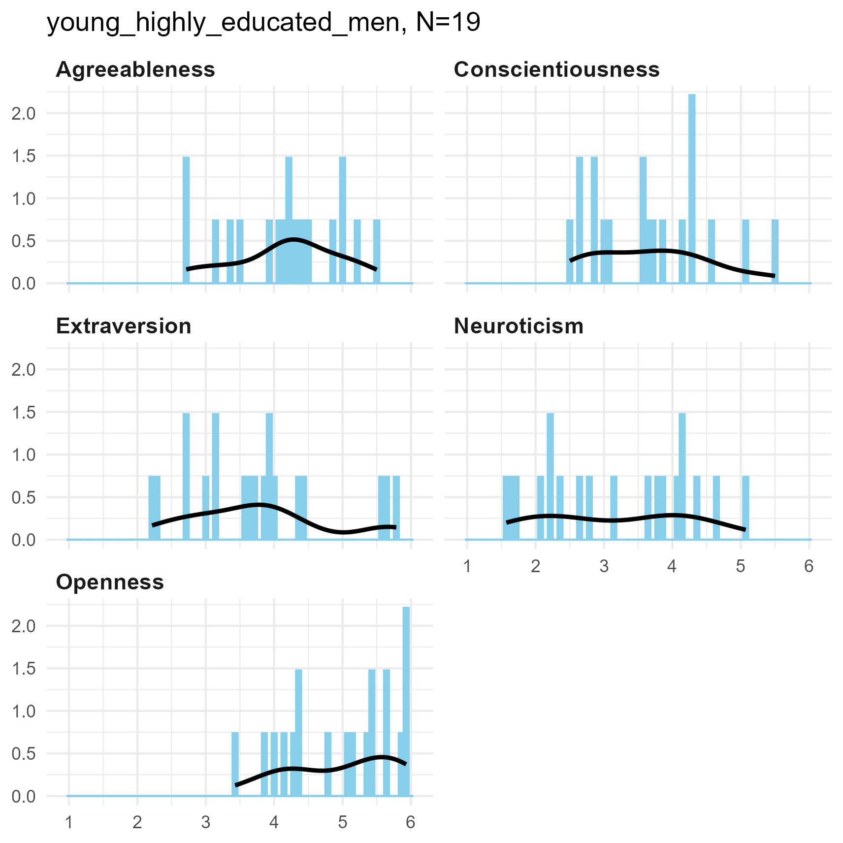
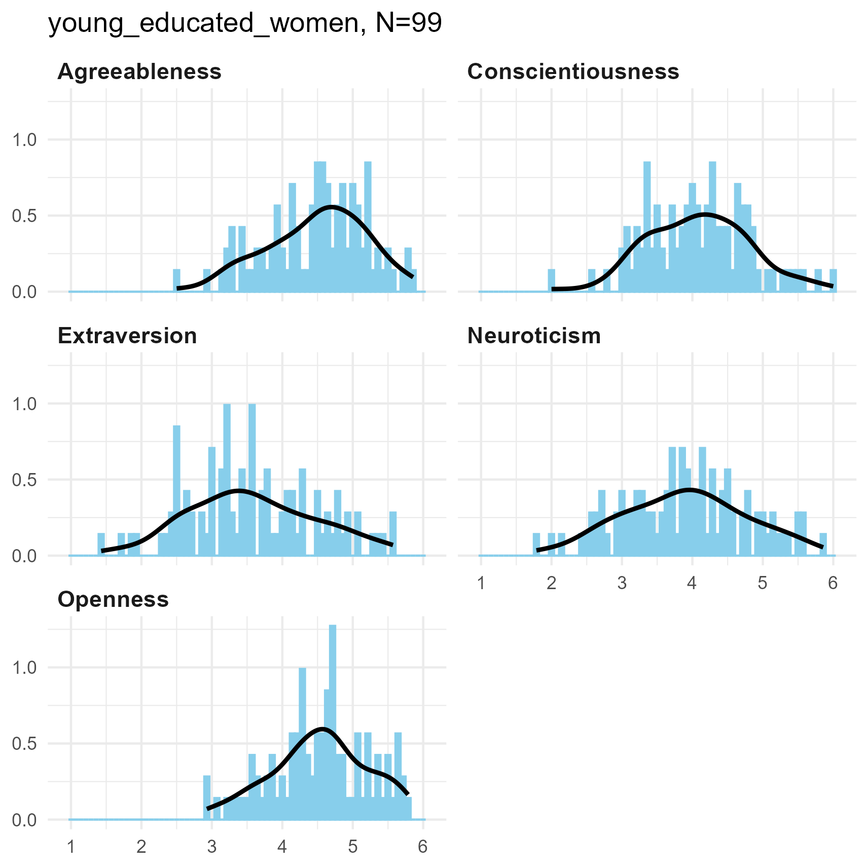
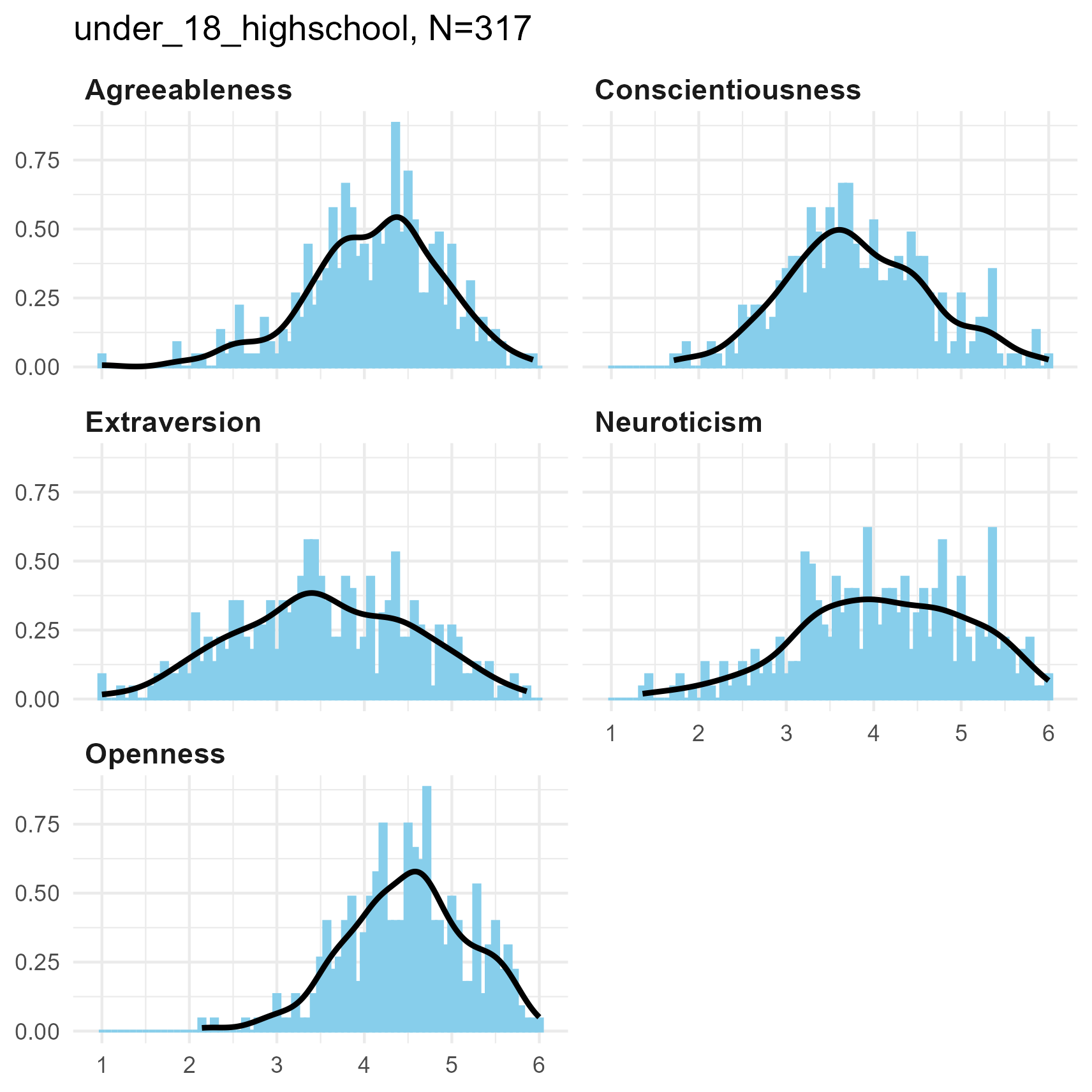
Big 5 Dimensions for three samples
SPI 27 Facets
Each of the SPI facets is the average of five six-point items, giving
5 * 6 = 30 potential values in each facet measure.
Again, the distributions tend to be unimodal, with smooth kernel density curves.
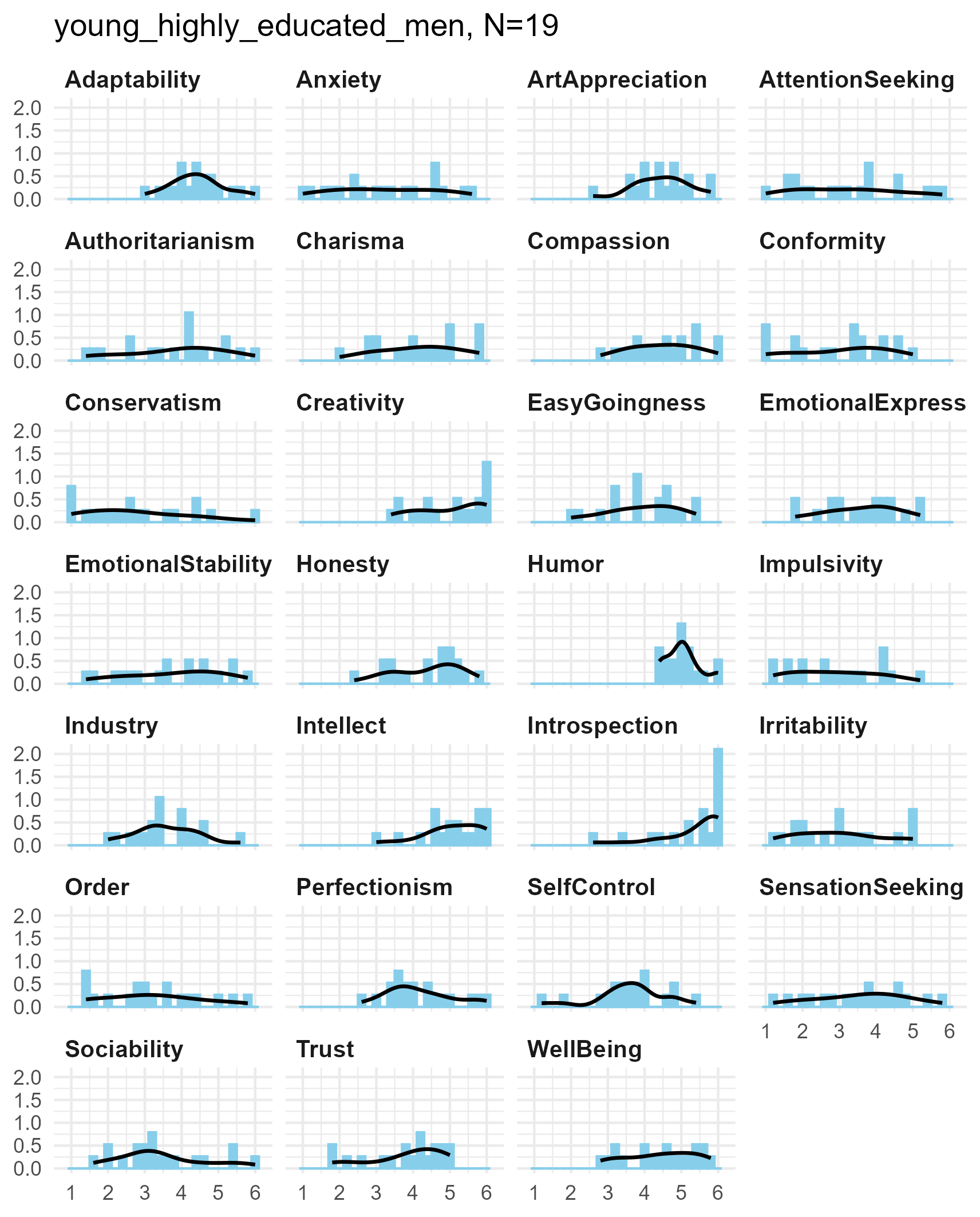
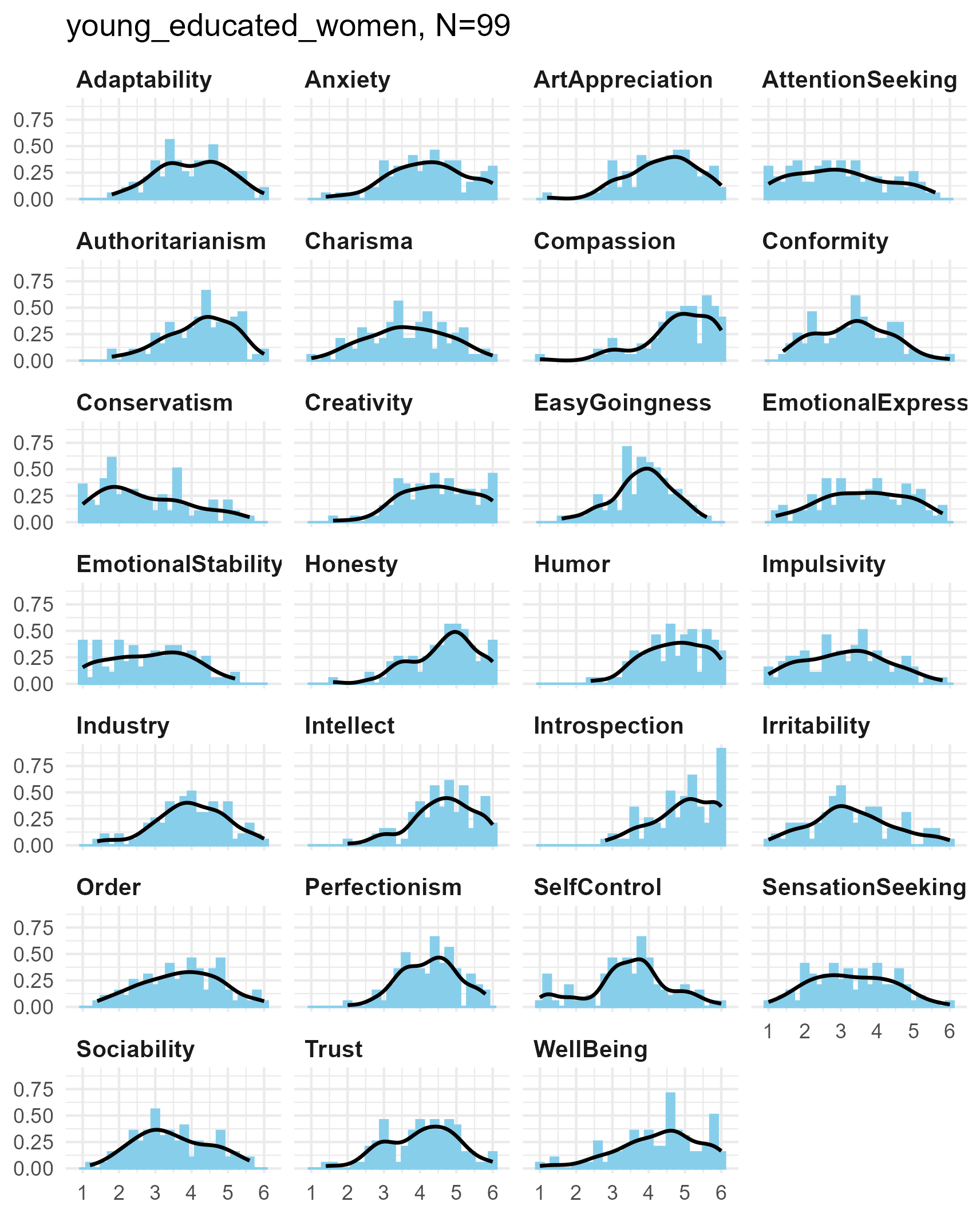
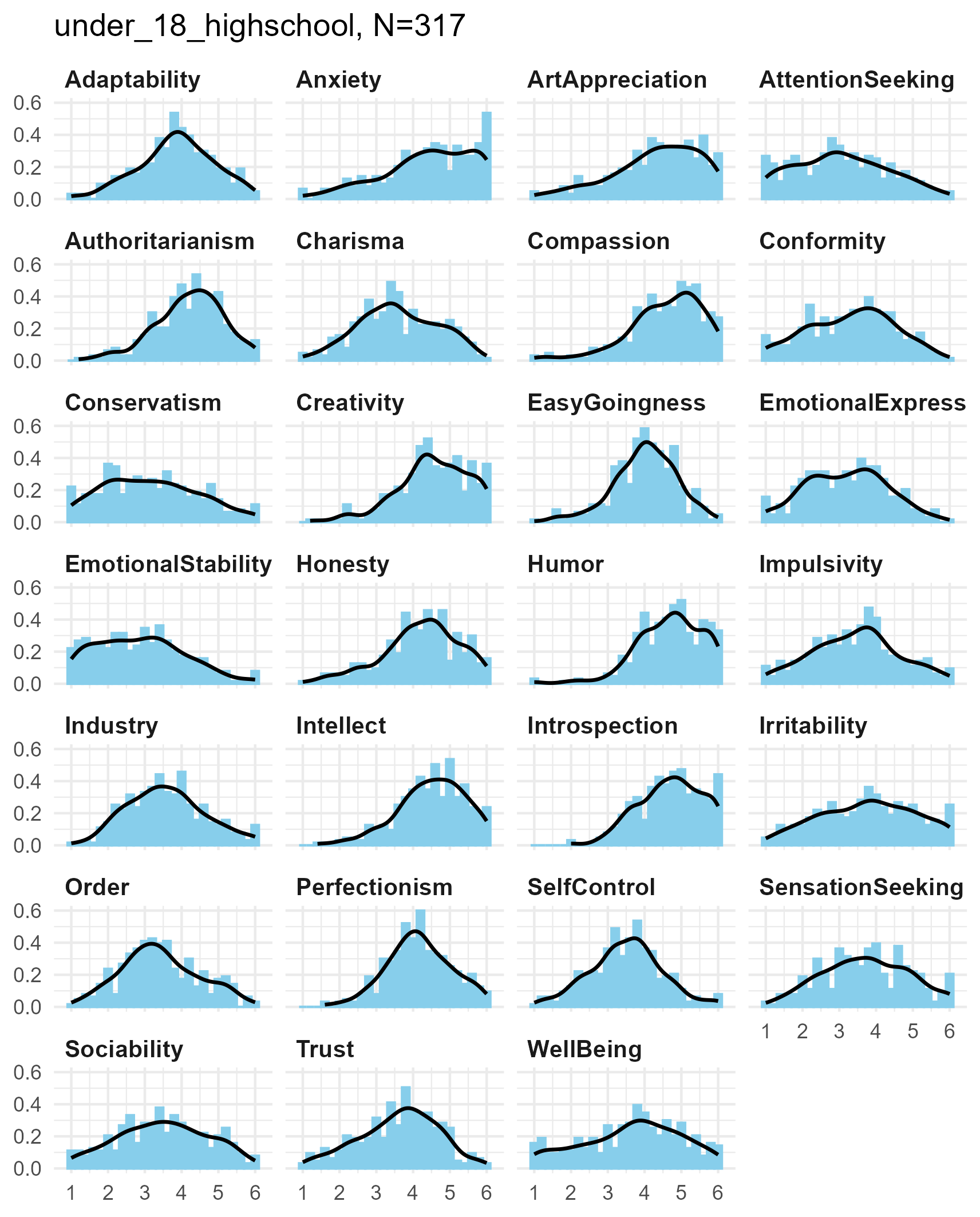
SPI facets for three samples
Selected SPI items
We simulated data for 135 individual items - too many to show meaningfully. We present here a sample of those few that showed unusual results in the simulations.
In these cases data were either highly skewed, or bimodal (or at least flat in parts).
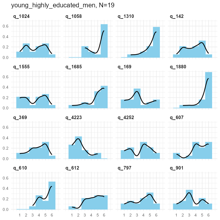
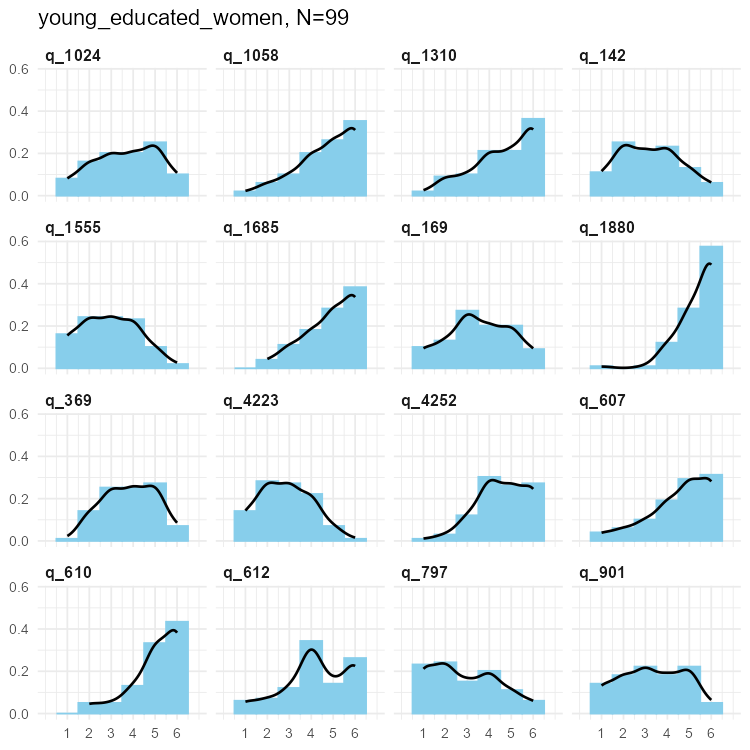
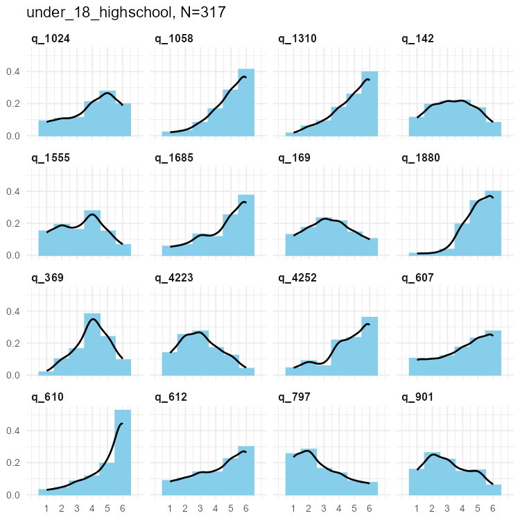
Selected SPI items for three samples
Results
The following tables list the dimension under consideration and the proportion of cases in each of the three samples that ere ‘statistically significant’ (\(\rho\) < 0.05).
Tables show the BWS test / Neuhäuser test.
Big Five Dimensions validity
Fourteen six-point items (84 levels in scale)
|
young men postgrad n=19 |
young women graduates n=99 |
under-18 highschool n=314 |
|
|---|---|---|---|
| Agreeableness | 0.00 / 0.00 | 0.00 / 0.00 | 0.00 / 0.00 |
| Conscientiousness | 0.00 / 0.00 | 0.00 / 0.00 | 0.01 / 0.00 |
| Extraversion | 0.00 / 0.00 | 0.00 / 0.00 | 0.00 / 0.00 |
| Neuroticism | 0.00 / 0.00 | 0.00 / 0.00 | 0.00 / 0.00 |
| Openness | 0.00 / 0.00 | 0.00 / 0.00 | 0.04 / 0.00 |
With smooth kernel density estimates, as we saw above, all
cases were non-significant, suggesting that such data are
well-reproduced by the LikertMakeR::lfast() function.
SPI Facets (Subscale) validity
Five six-point items (30 potential values in scale)
|
young men postgrad n=19 |
young women graduates n=99 |
under-18 highschool n=314 |
|
|---|---|---|---|
| Adaptability | 0.00 / 0.00 | 0.00 / 0.00 | 1.00 / 0.00 |
| Anxiety | 0.00 / 0.00 | 0.01 / 0.00 | 1.00 / 0.00 |
| ArtAppreciation | 0.00 / 0.00 | 0.00 / 0.00 | 1.00 / 0.00 |
| AttentionSeeking | 0.00 / 0.00 | 0.00 / 0.00 | 1.00 / 0.03 |
| Authoritarianism | 0.00 / 0.00 | 0.00 / 0.00 | 1.00 / 0.00 |
| Charisma | 0.00 / 0.00 | 0.00 / 0.00 | 1.00 / 0.00 |
| Compassion | 0.00 / 0.00 | 0.86 / 0.00 | 1.00 / 0.00 |
| Conformity | 0.00 / 0.00 | 0.00 / 0.00 | 1.00 / 0.00 |
| Conservatism | 0.00 / 0.00 | 0.09 / 0.00 | 1.00 / 0.00 |
| Creativity | 0.00 / 0.00 | 0.10 / 0.00 | 1.00 / 0.00 |
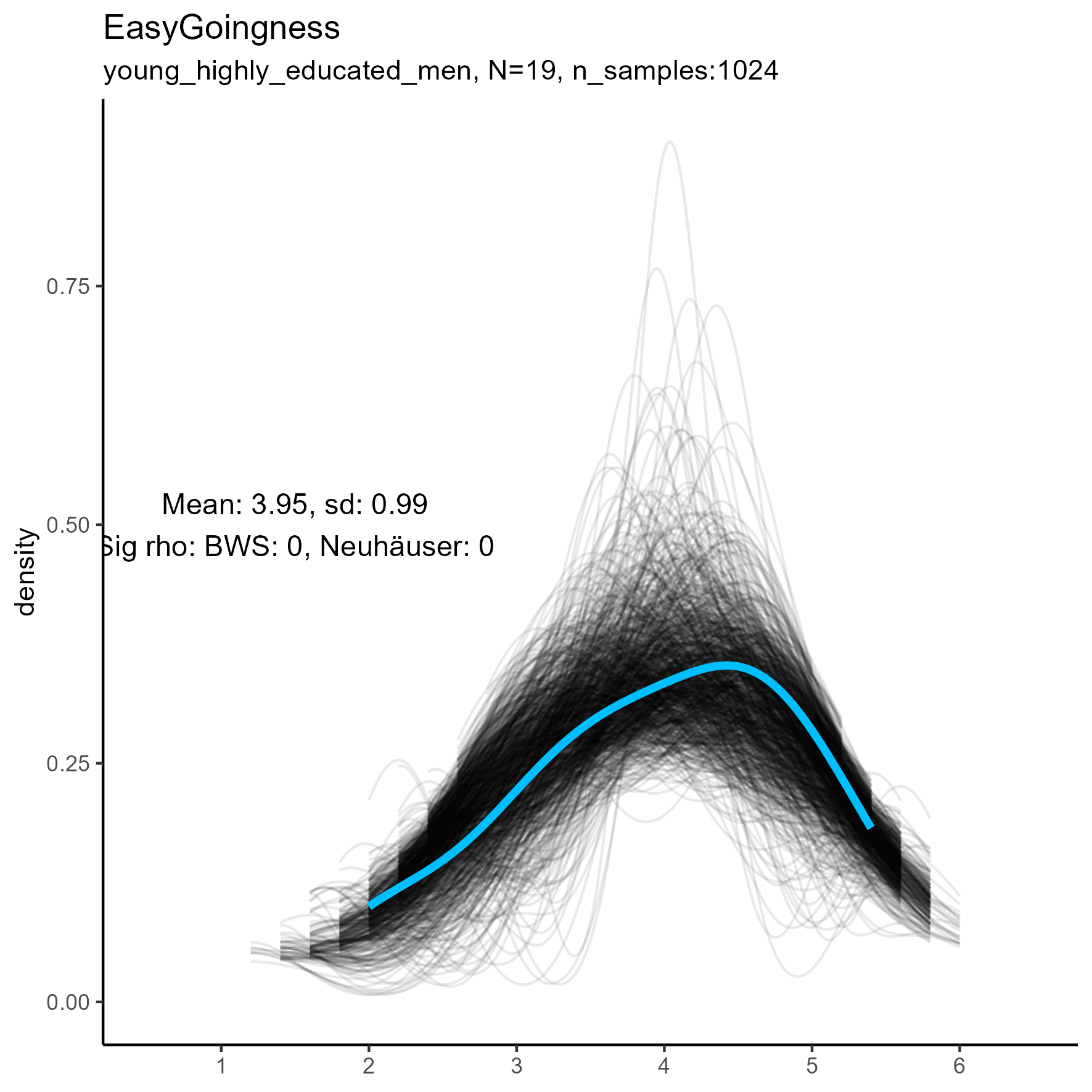
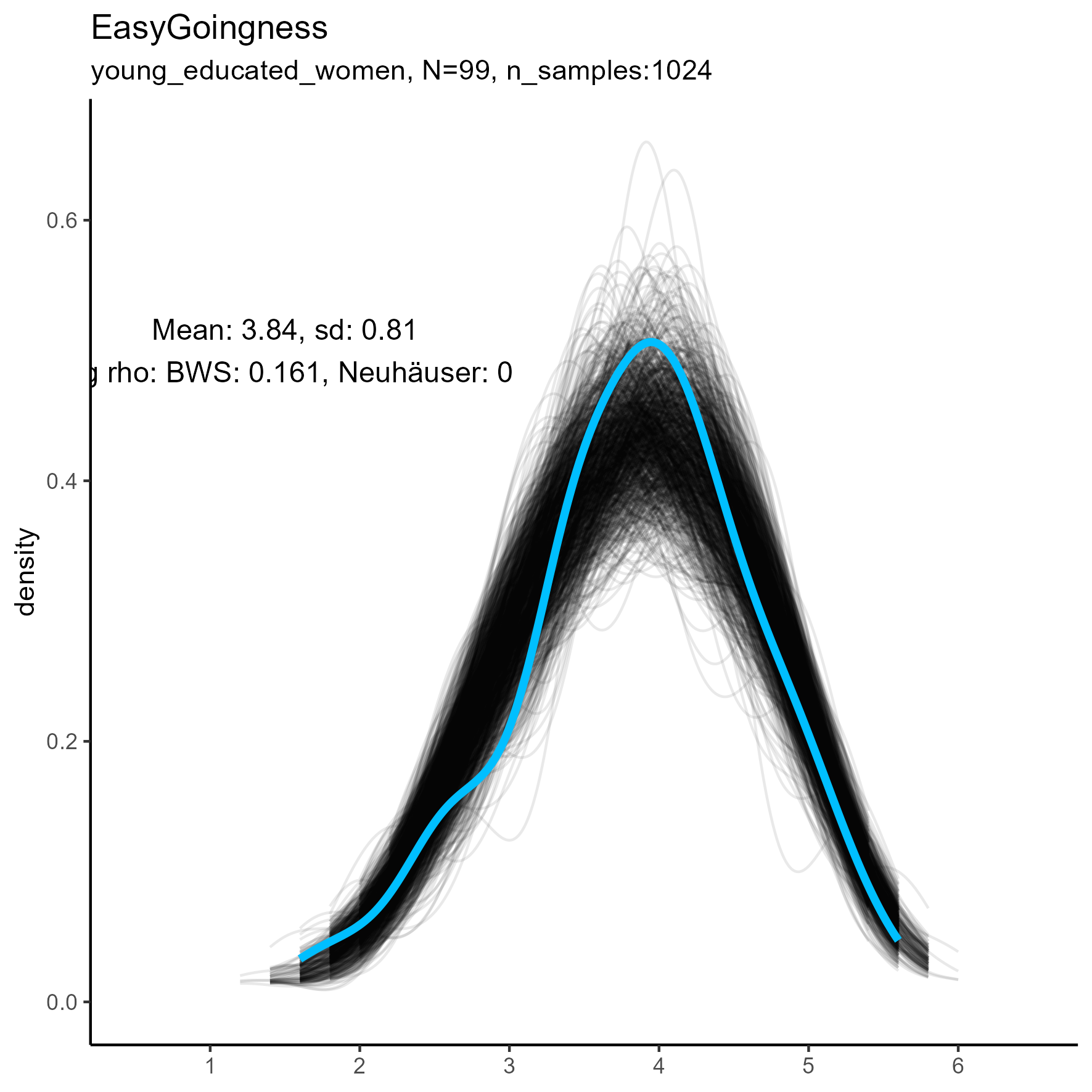
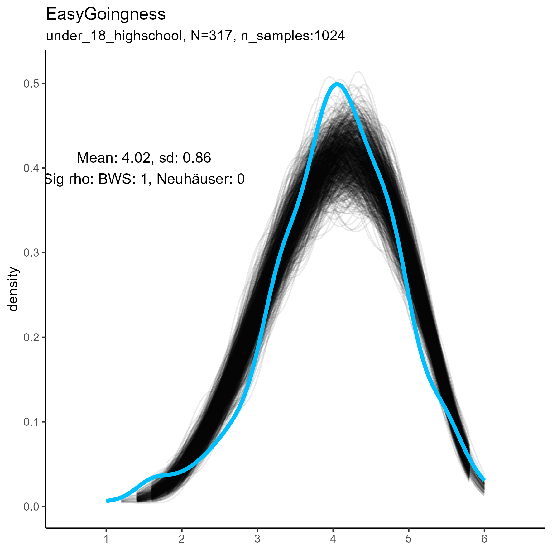
| EasyGoingness | 0.00 / 0.00 | 0.16 / 0.00 | 1.00 / 0.00 |
| EmotionalExpressiveness | 0.00 / 0.00 | 0.00 / 0.00 | 1.00 / 0.00 |
| EmotionalStability | 0.00 / 0.00 | 0.08 / 0.00 | 1.00 / 0.04 |
| Honesty | 0.00 / 0.00 | 0.05 / 0.00 | 1.00 / 0.00 |
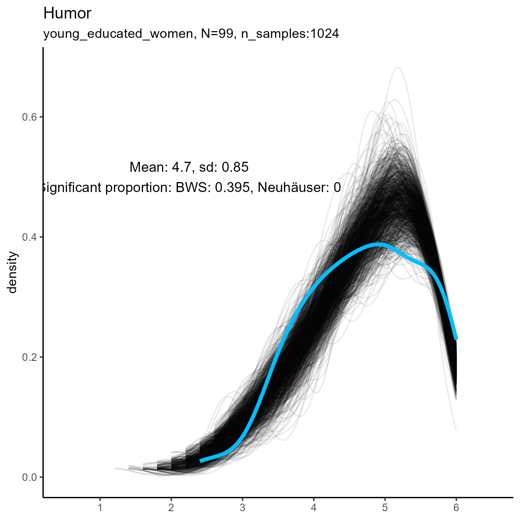
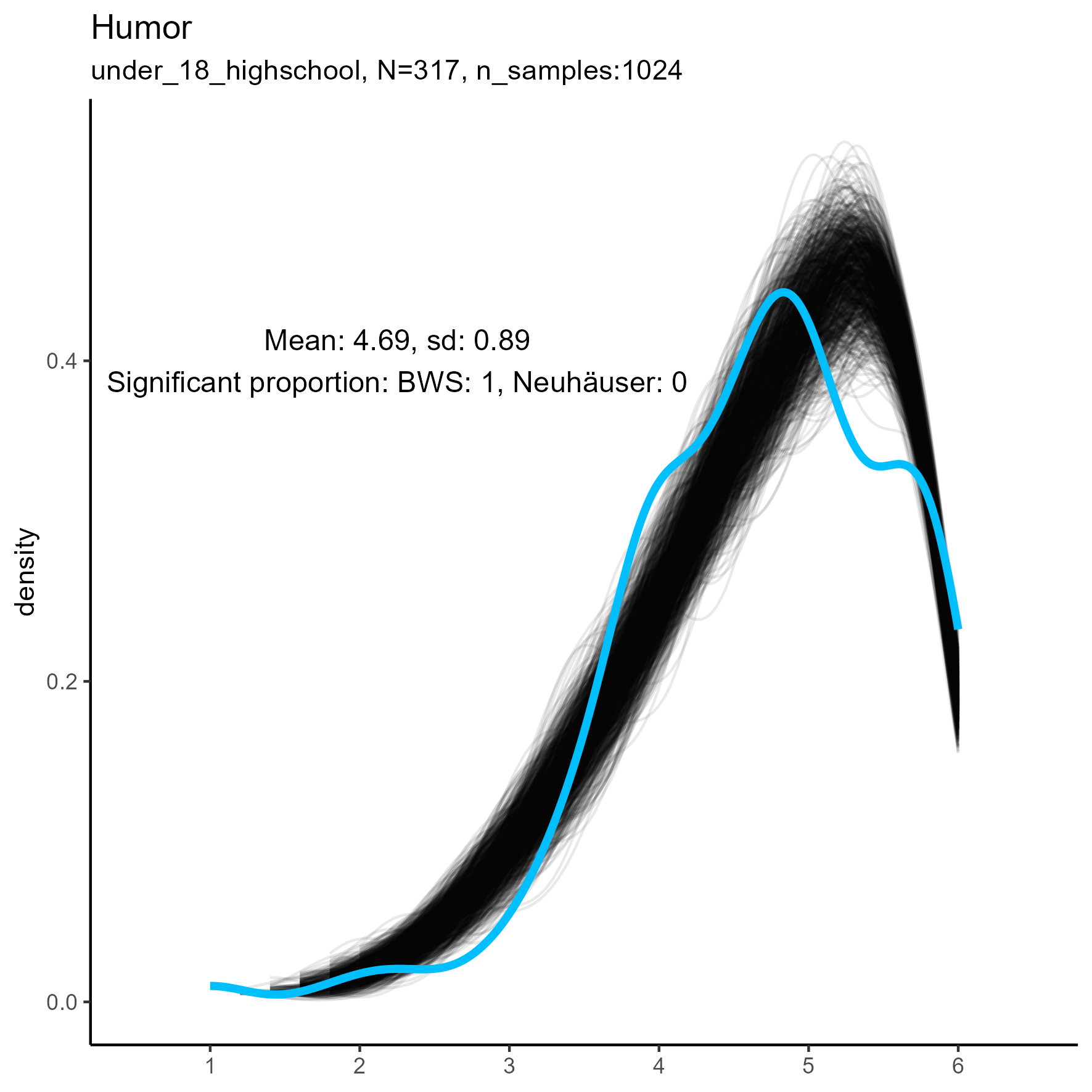
| Humor | 0.02 / 0.01 | 0.40 / 0.00 | 1.00 / 0.00 |
| Impulsivity | 0.00 / 0.00 | 0.00 / 0.00 | 1.00 / 0.00 |
| Industry | 0.00 / 0.00 | 0.00 / 0.00 | 1.00 / 0.00 |
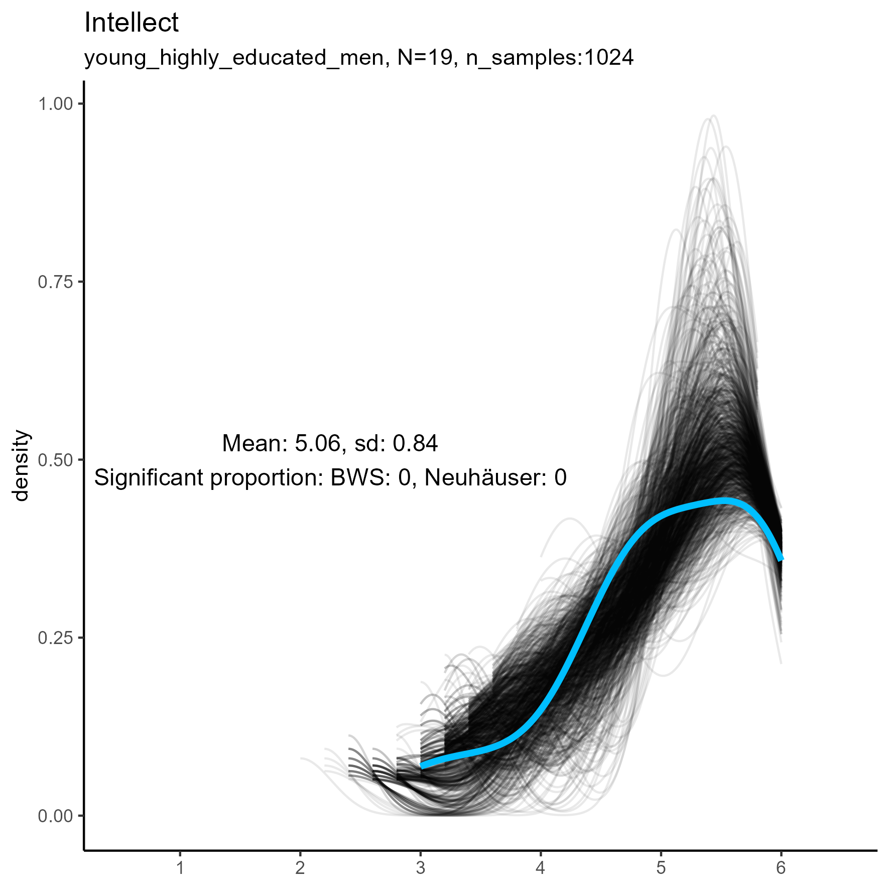
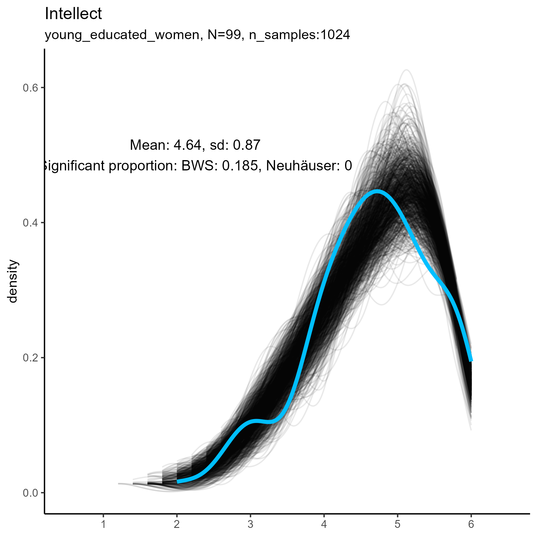
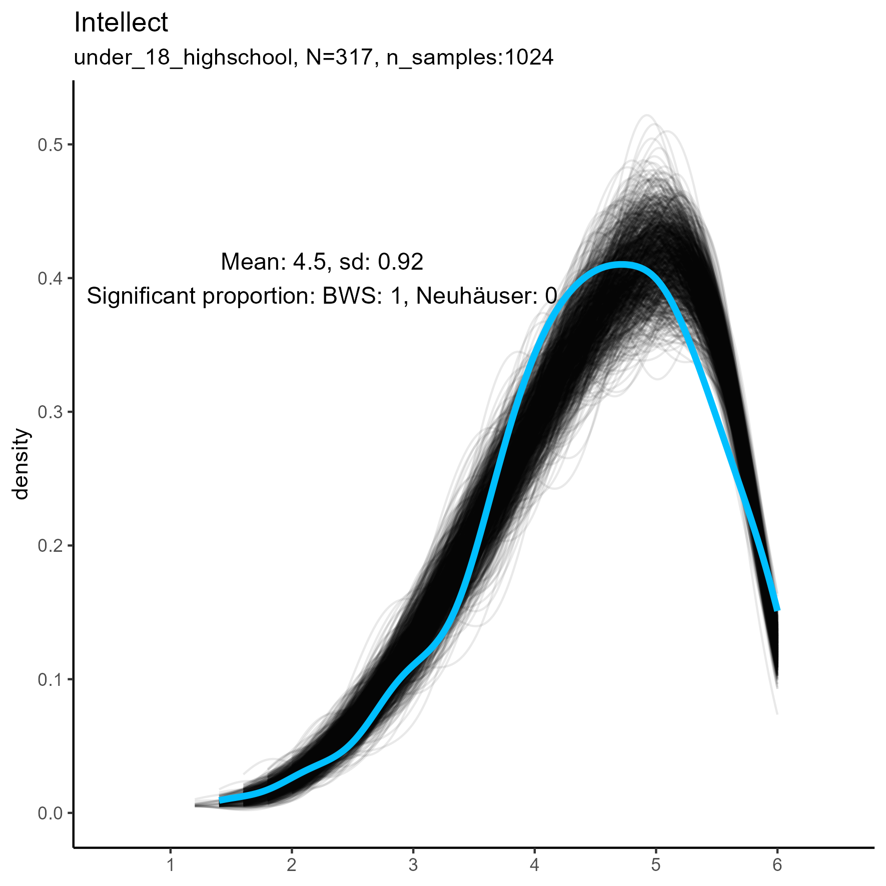
| Intellect | 0.00 / 0.00 | 0.22 / 0.00 | 1.00 / 0.00 |
| Introspection | 0.99 / 0.00 | 1.00 / 0.00 | 1.00 / 0.00 |
| Irritability | 0.00 / 0.00 | 0.00 / 0.00 | 1.00 / 0.00 |
| Order | 0.00 / 0.00 | 0.00 / 0.00 | 1.00 / 0.00 |
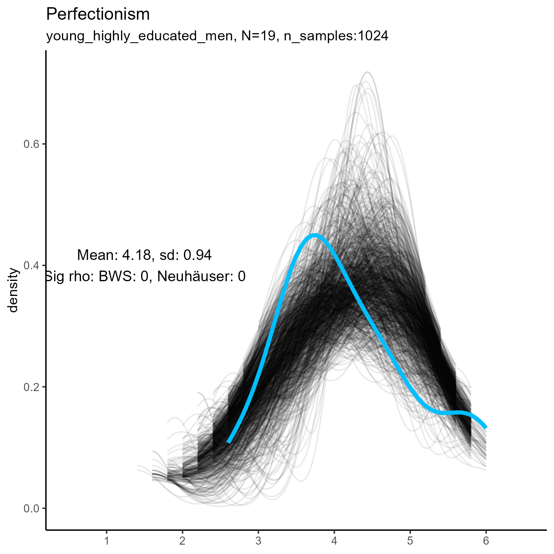
| Perfectionism | 0.00 / 0.00 | 0.15 / 0.00 | 1.00 / 0.00 |
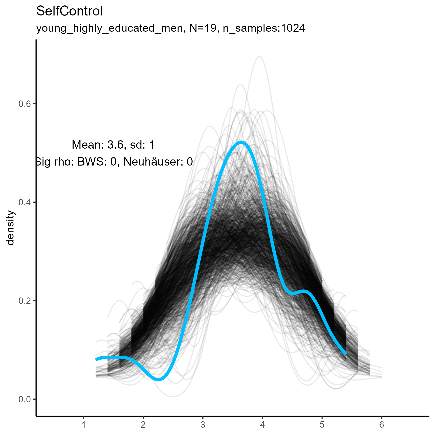
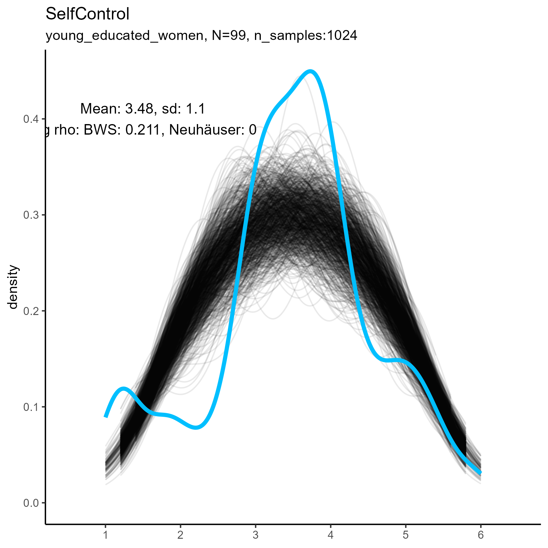
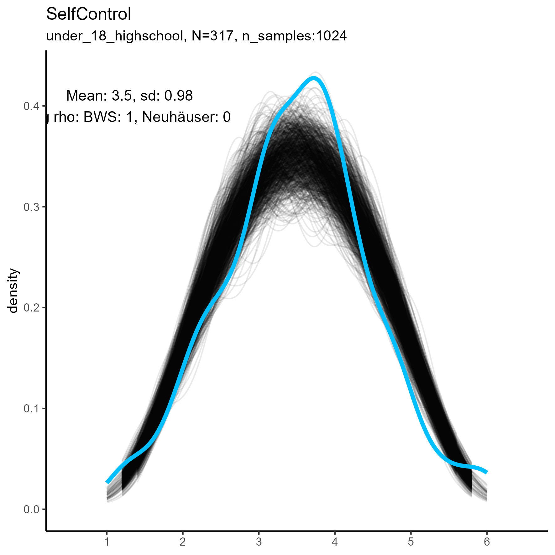
| SelfControl | 0.00 / 0.00 | 0.19 / 0.00 | 1.00 / 0.00 |
| SensationSeeking | 0.00 / 0.00 | 0.00 / 0.00 | 1.00 / 0.00 |
| Sociability | 0.00 / 0.00 | 0.00 / 0.00 | 1.00 / 0.00 |
| Trust | 0.00 / 0.00 | 0.00 / 0.00 | 1.00 / 0.00 |
| WellBeing | 0.00 / 0.00 | 0.00 / 0.00 | 1.00 / 0.00 |
When the BWS test is applied to the larger sample, all simulations are significantly different from the original data. This is probably due to the smaller standard error produced by a larger sample.
Interestingly, the Neuhäuser test, which is less sensitive to outliers, suggested that all simulations are good representations of the original.
The facet, Introspection, stands out as one that is rarely
accurately reproduced by the LikertMakeR::lfast() function,
using the BWS test, regardless of sample size.
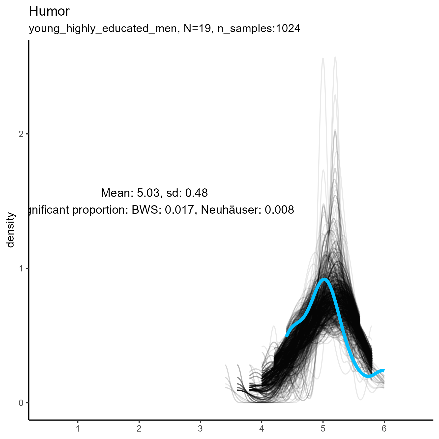
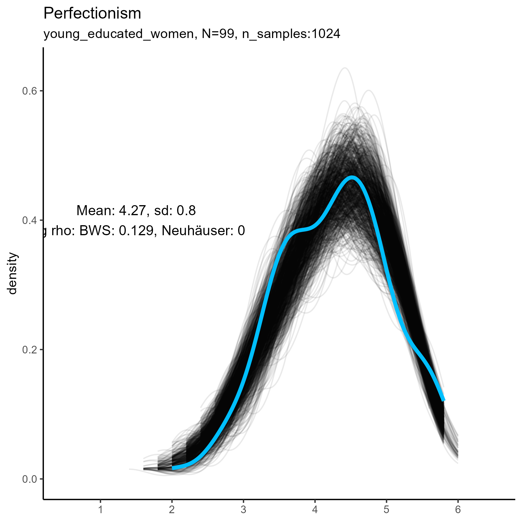
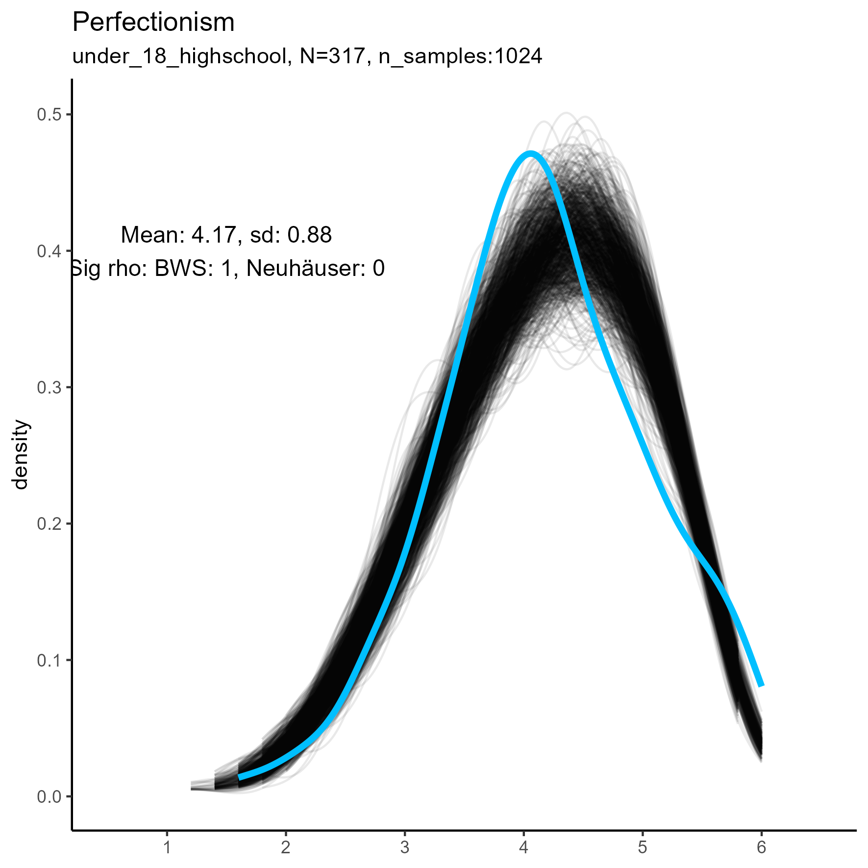
Other facets that are worth exploring in more detail are: Compassion, Humor, Intellect, SelfControl, EasyGoingness, and Perfectionism. These facets have high rates of significance in the mid-sample-size condition.
Focus on “Introspection” facet
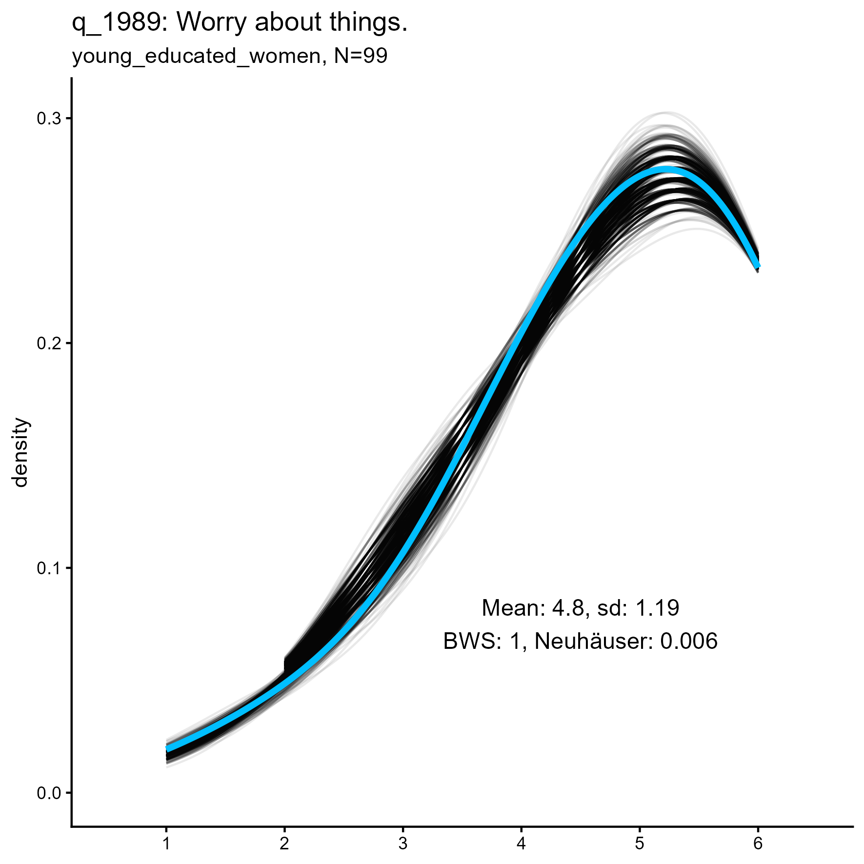
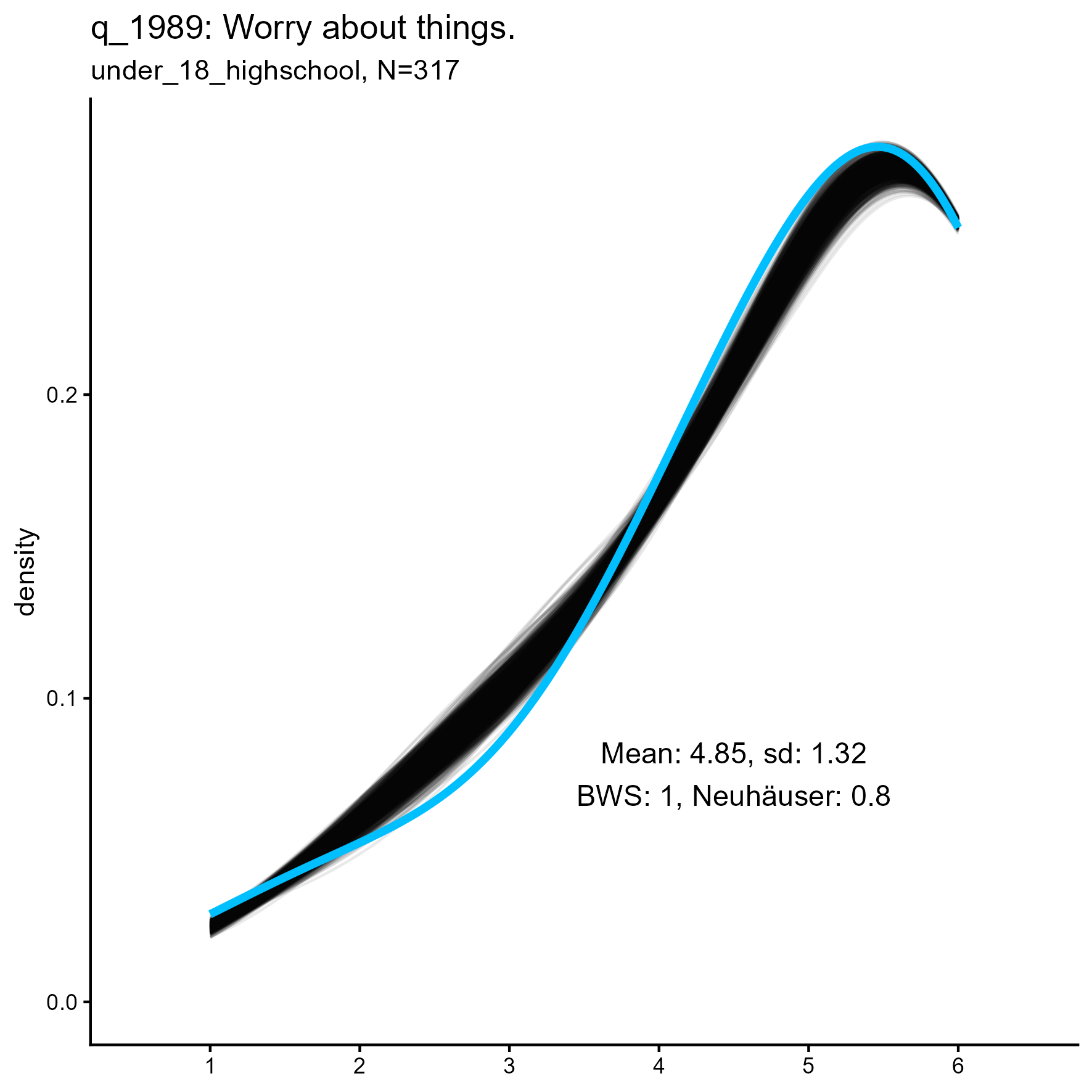
The following chart shows kernel density plots for facet Introspection in the three samples.
Each of the 1024 synthetic dataframes is represented by a grey/black line, and the original “true” dataframe is represented by a blue/cyan line.
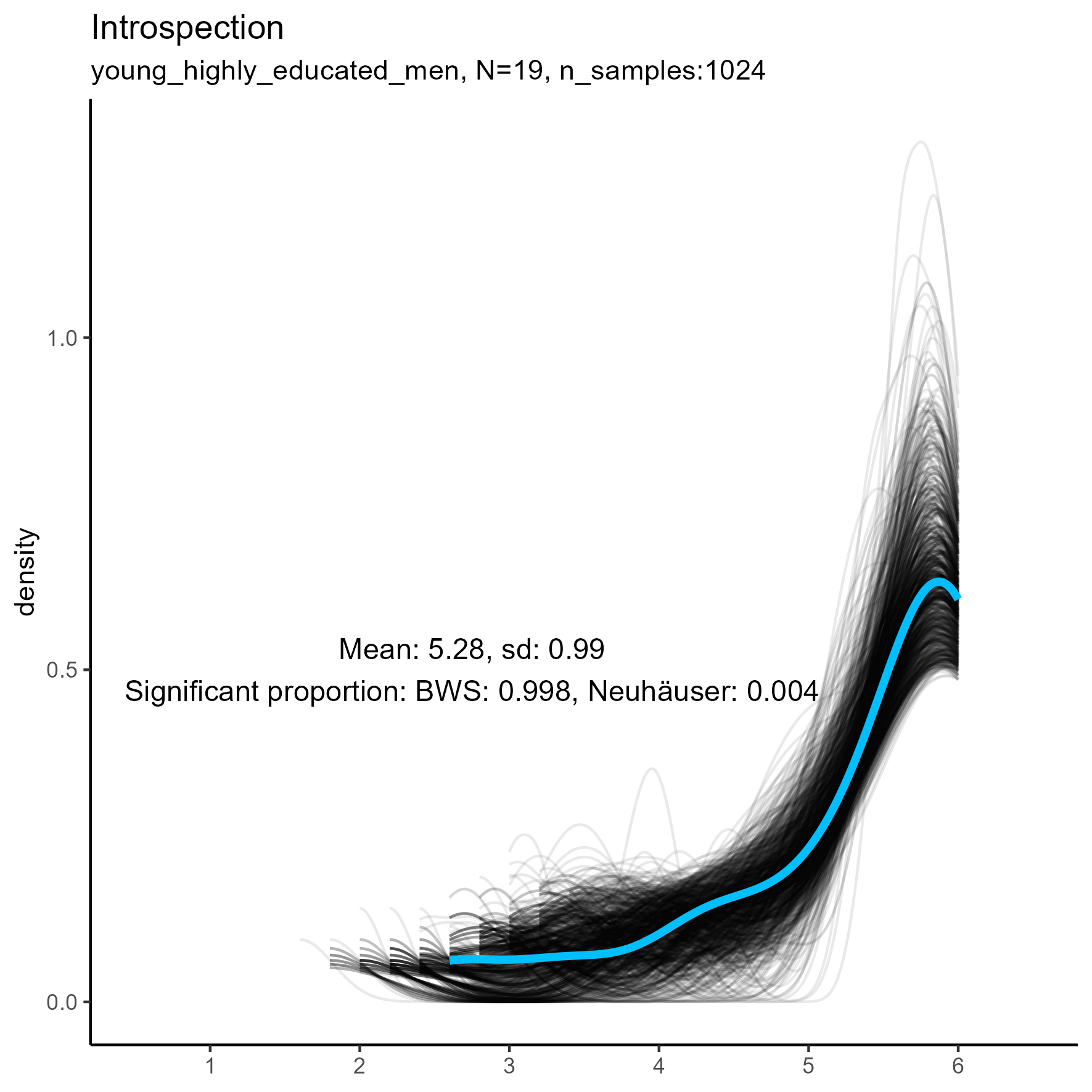
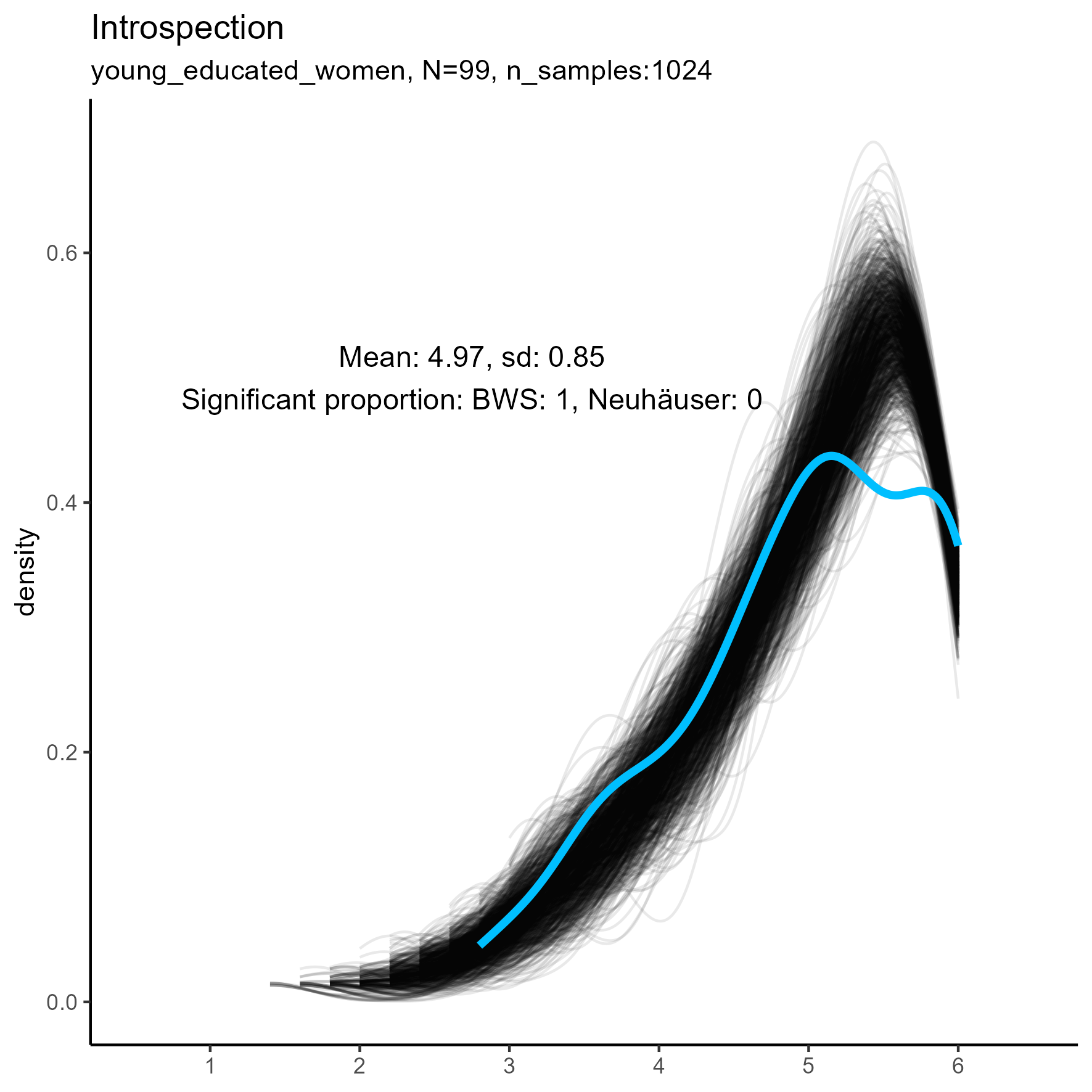
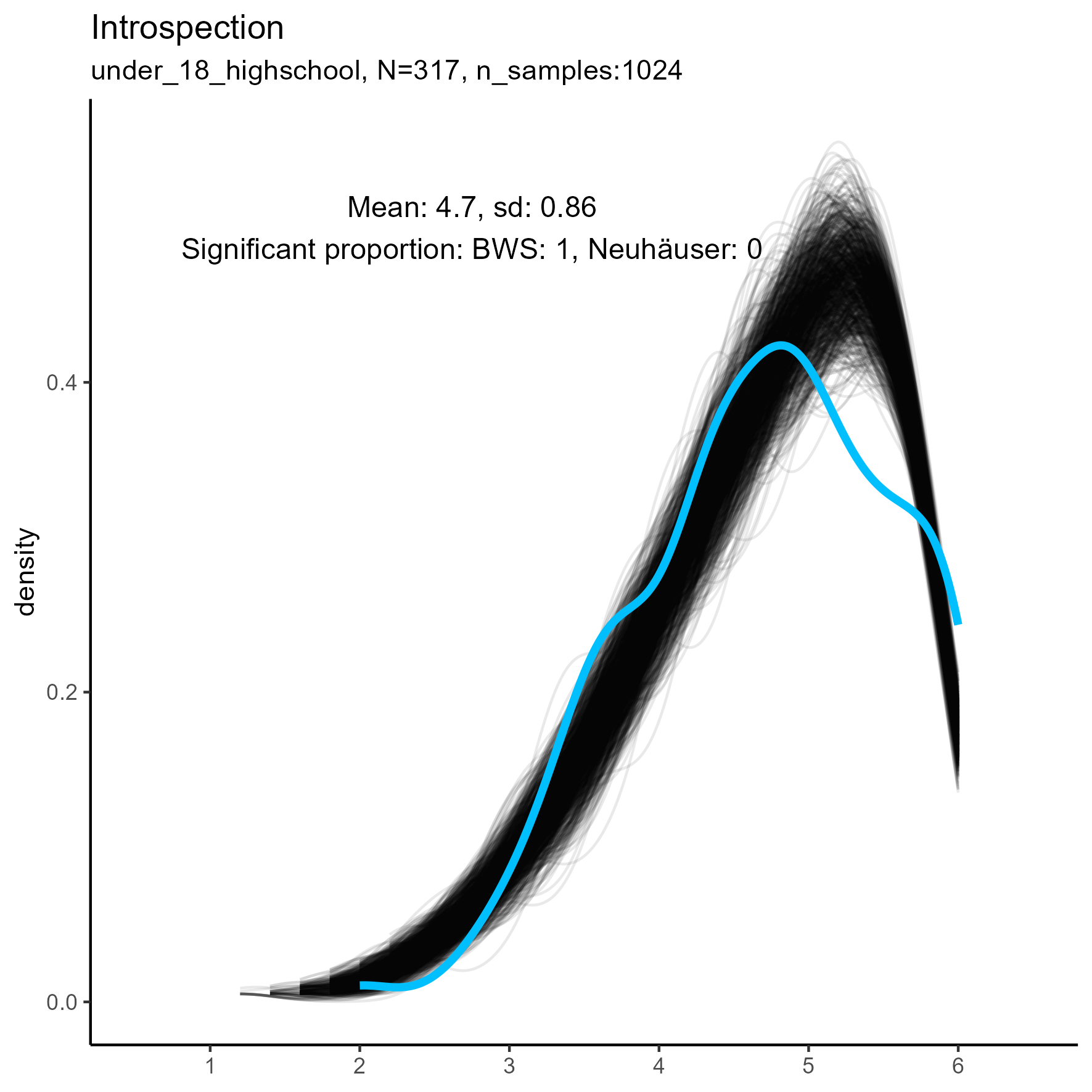
Introspection facet: Density plot for small, medium and large samples
We see that the synthetic data never match the true data, especially in the middle and large sample sizes.
The original, true, data are highly left-skewed, and this has been nicely captured by the synthetic data. Note, however, that the true dataframe is not unimodal. The kernel density estimate appears rough and slightly multimodal. It’s more wobbly.
focus on “Compassion” facet
The following chart shows kernel density plots for facet Compassion in the three samples.
Again, each of the 1024 synthetic dataframes is represented by a grey/black line, and the original “true” dataframe is represented by a blue/cyan line.
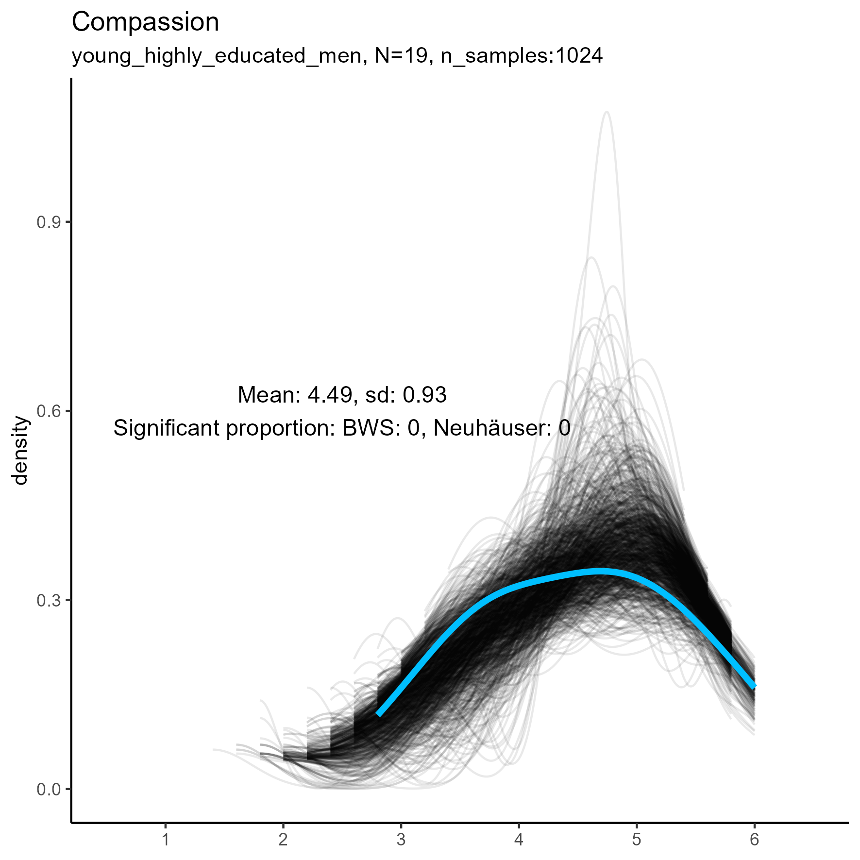
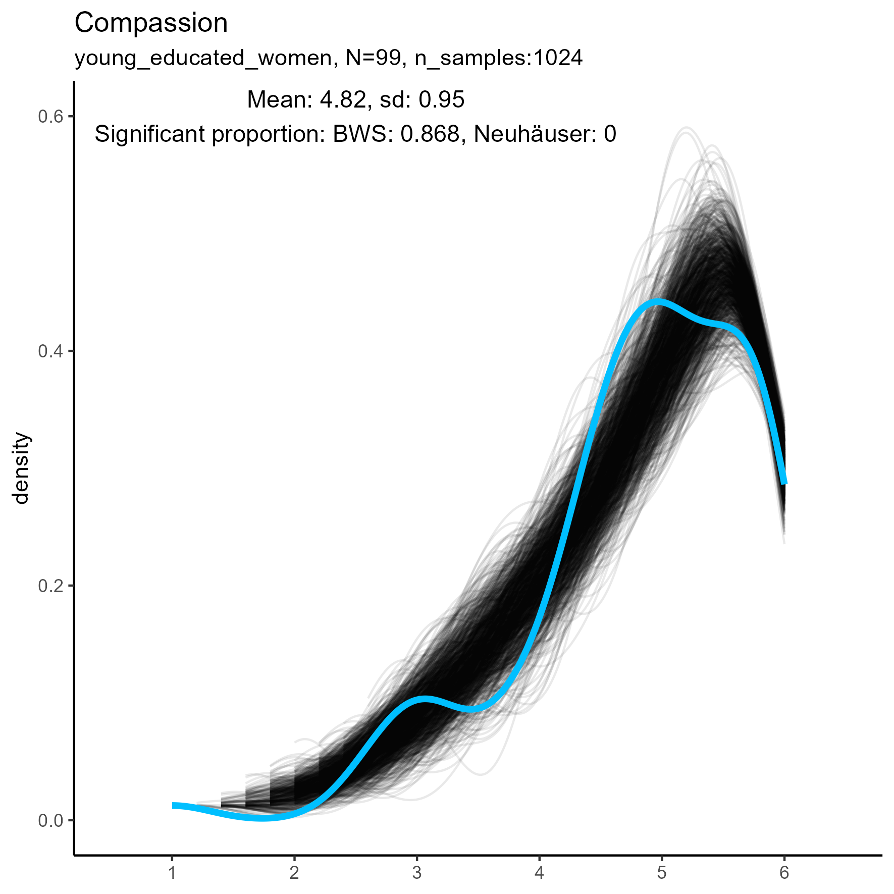
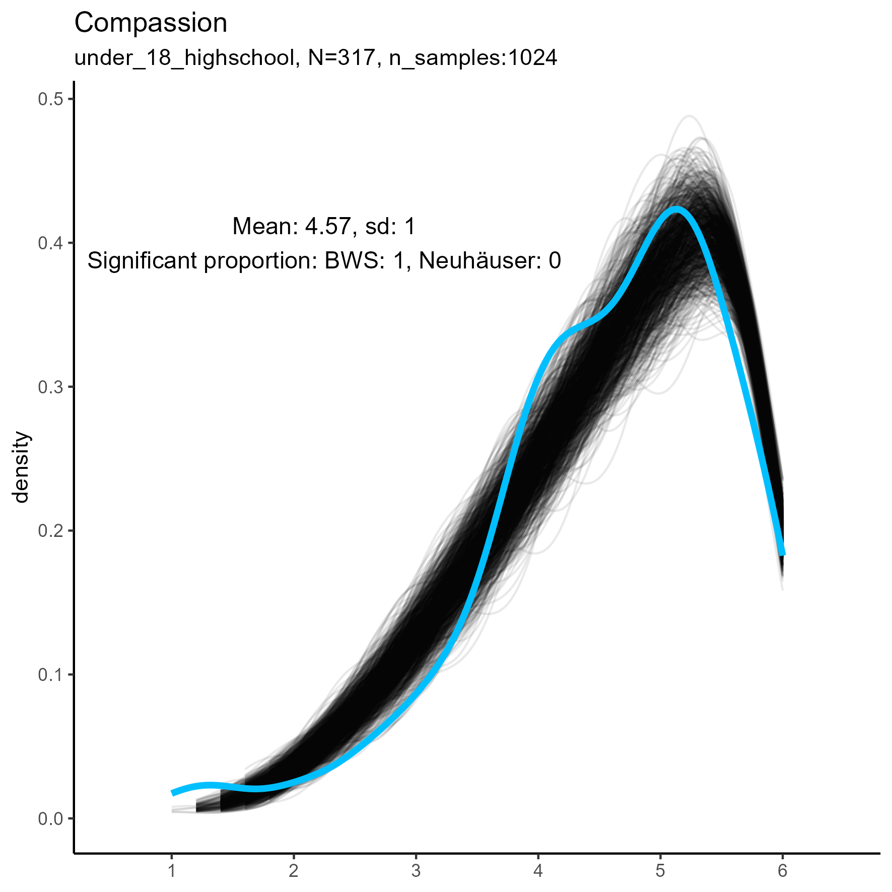
Compassion facet: Kernel Density plots for small, medium and large samples
For this factor the BWS test showed no cases where the synthetic data were significantly different from the original data for the smaller sample. But for the medium and large samples, the original data are not unimodal, and the BWS test suggests that all synthetic replications are different from the original.
SPI Item validity
Each scale is a single six-point item.
In almost all cases, the Baumgartner–Weiß–Schindler (BWS) test showed a statistically significant difference between actual data and synthetic data. In most cases, however, the Neuhäuser test, which is more robust to outliers, was not statistically significant.
The appendix table shows summary results for the three data sets for all 135 items, indicating the proportion of cases where distribution comparison tests were ‘statistically significant’ (\(\rho\) < 0.05).
In about 37 of the 135 items (27%) did the BWS test show proportion of significant simulations less than 80%.
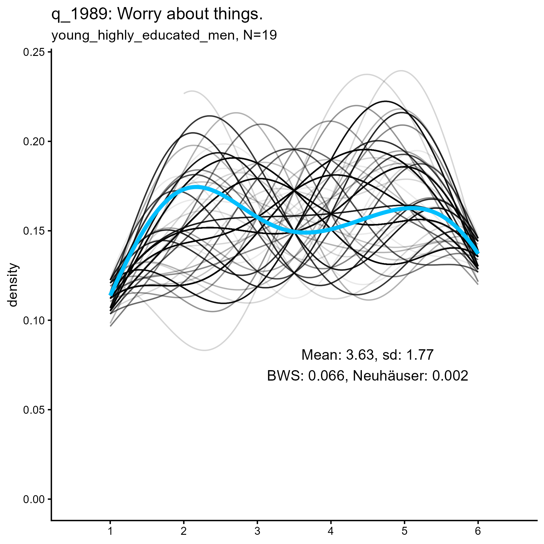
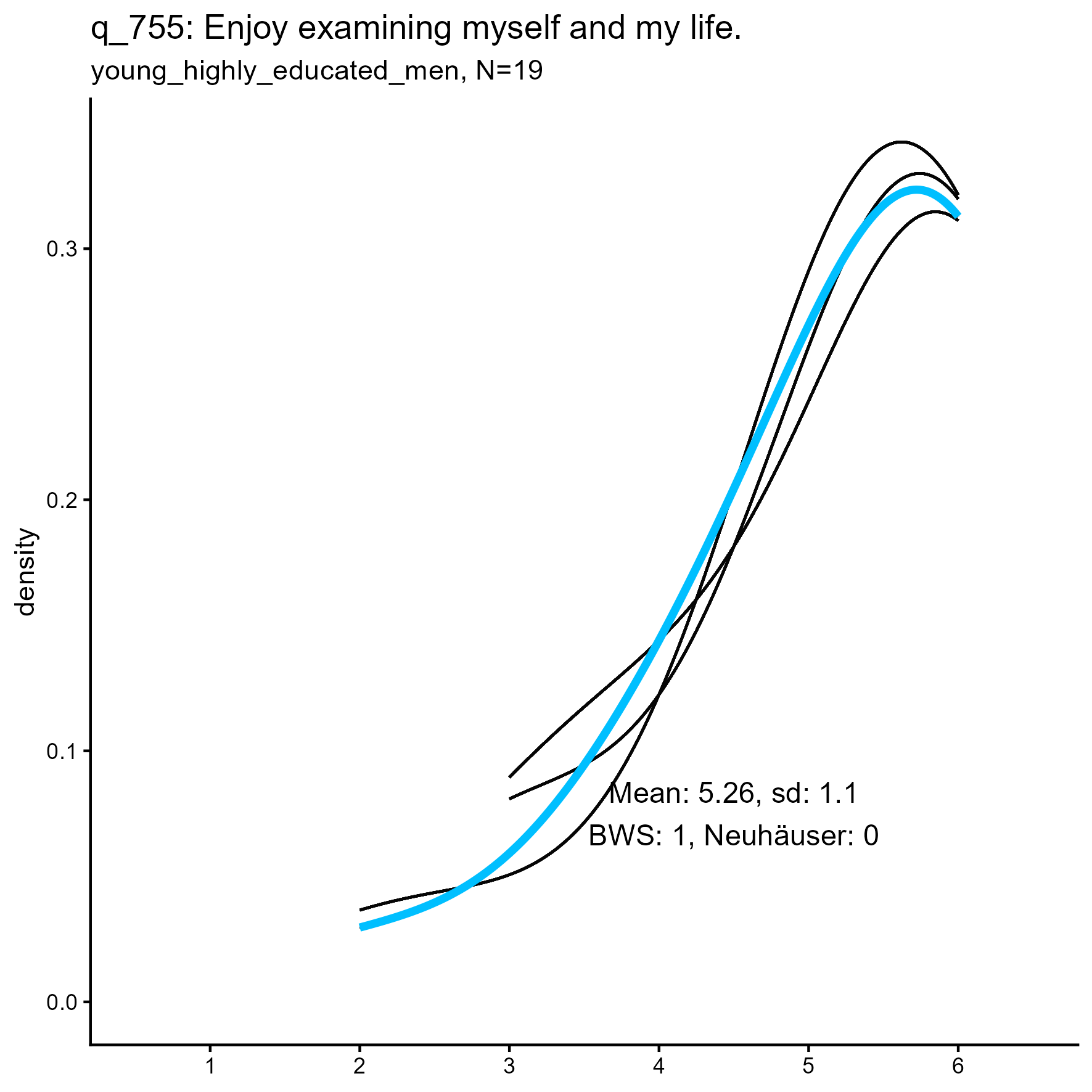
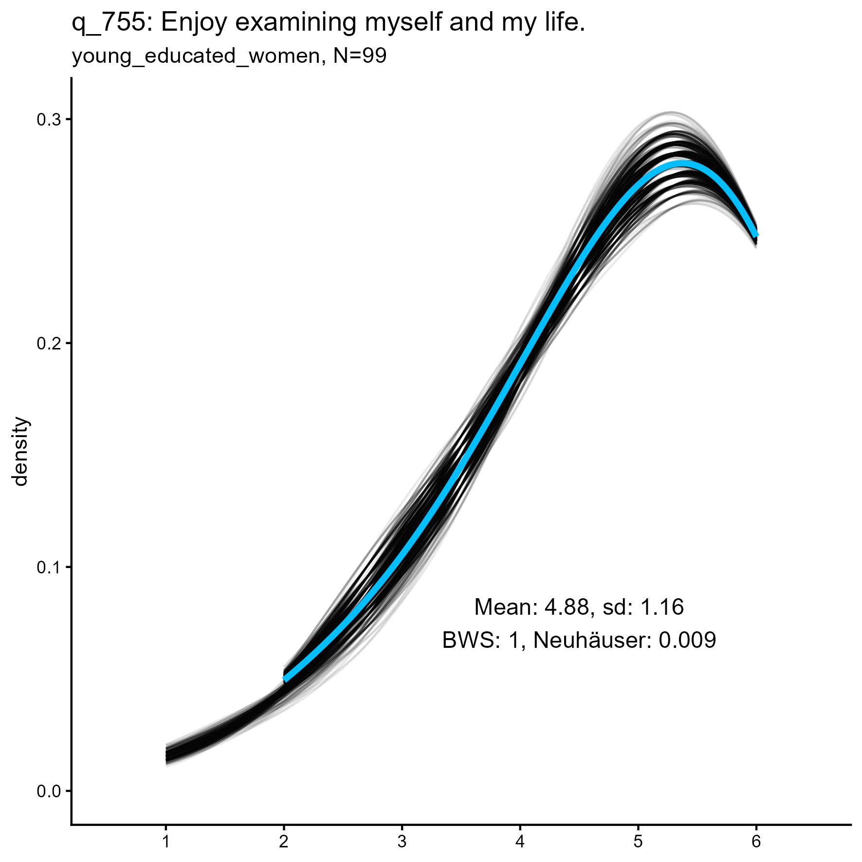
The following are some sample item results for each of the three samples
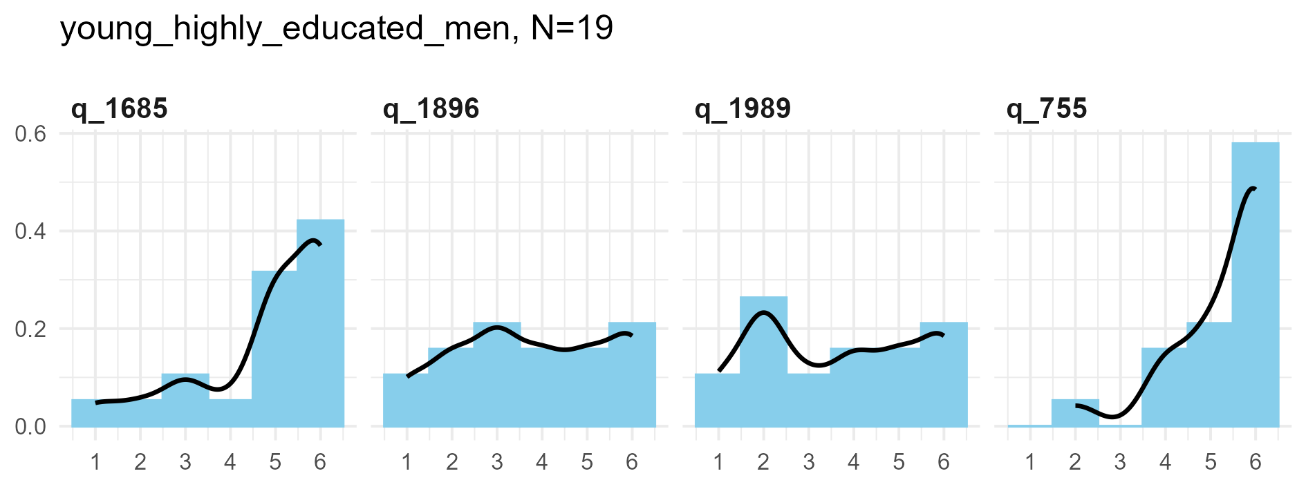
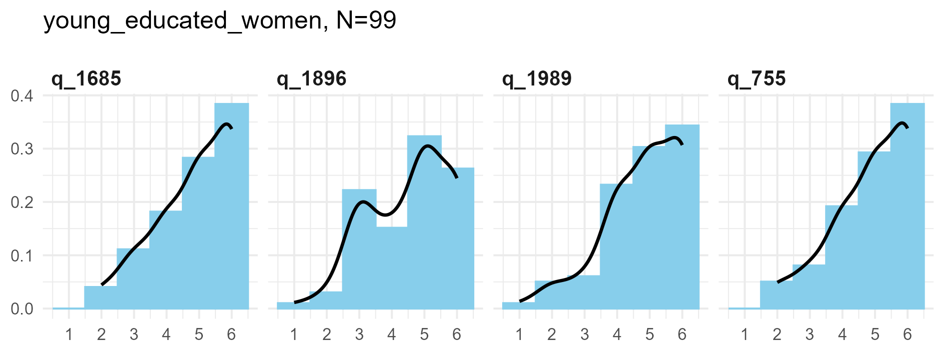
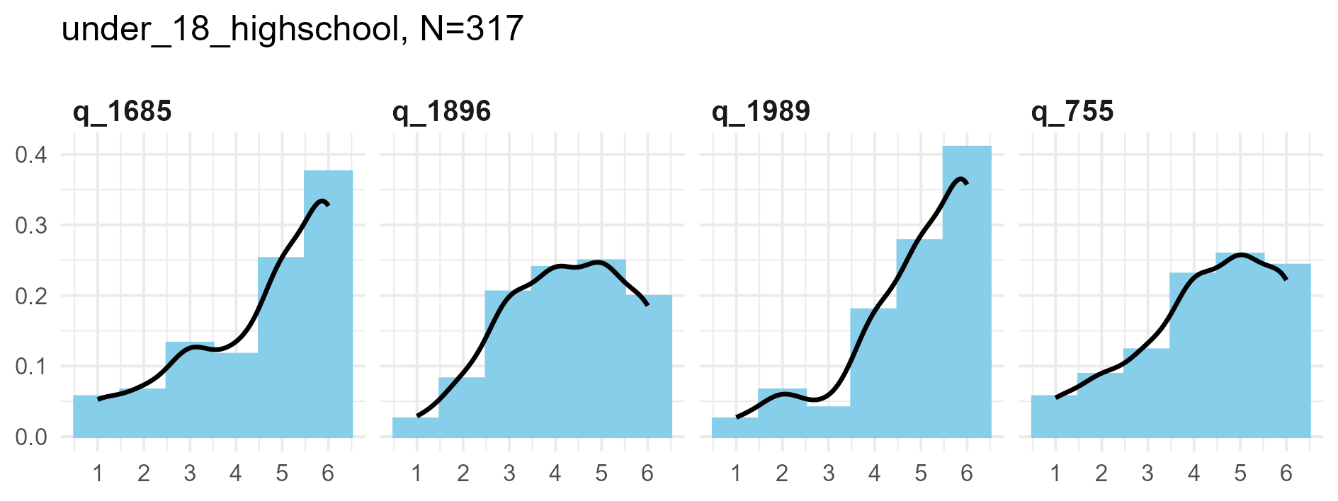
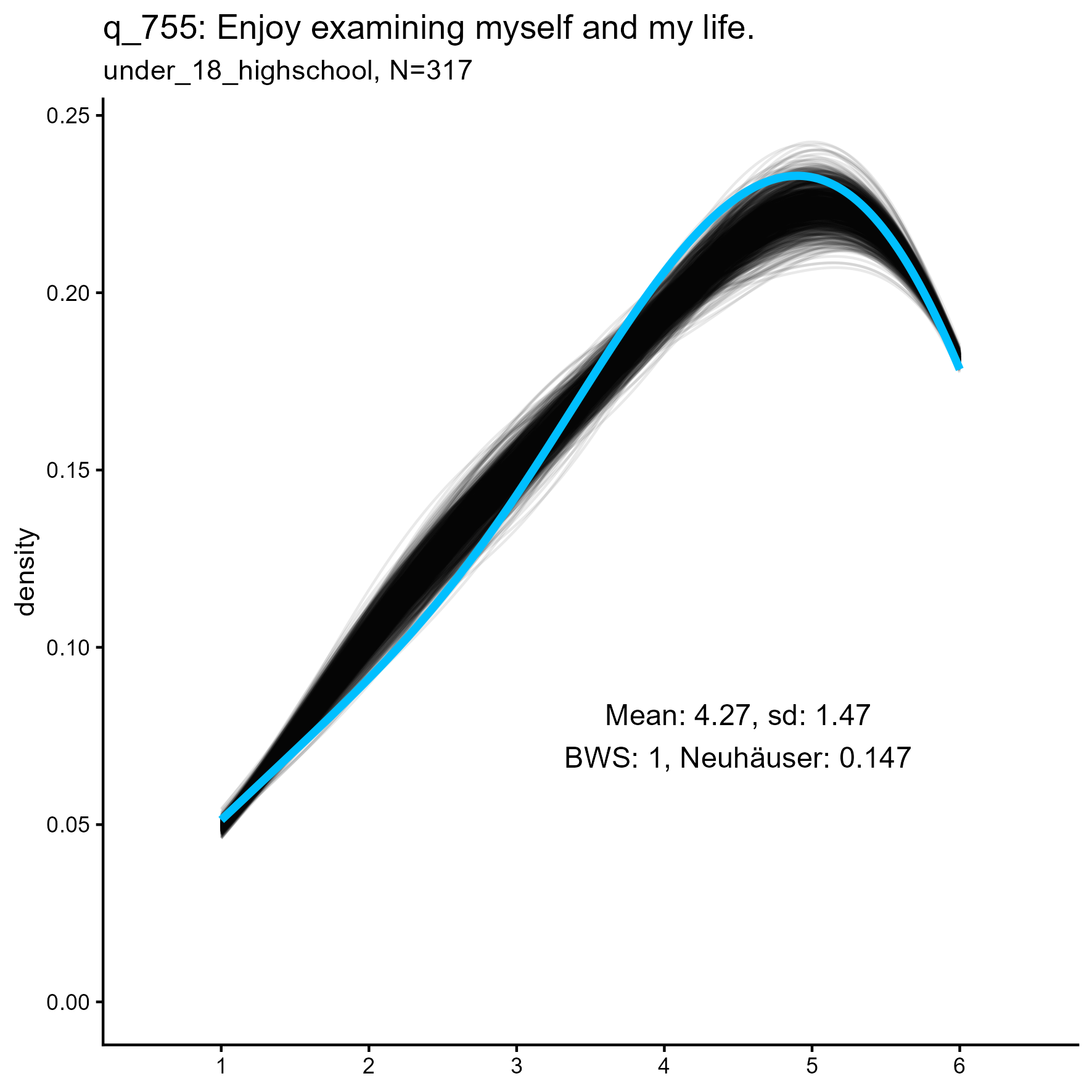
Synthetic data density plots
q_1685 ‘Seldom joke around’
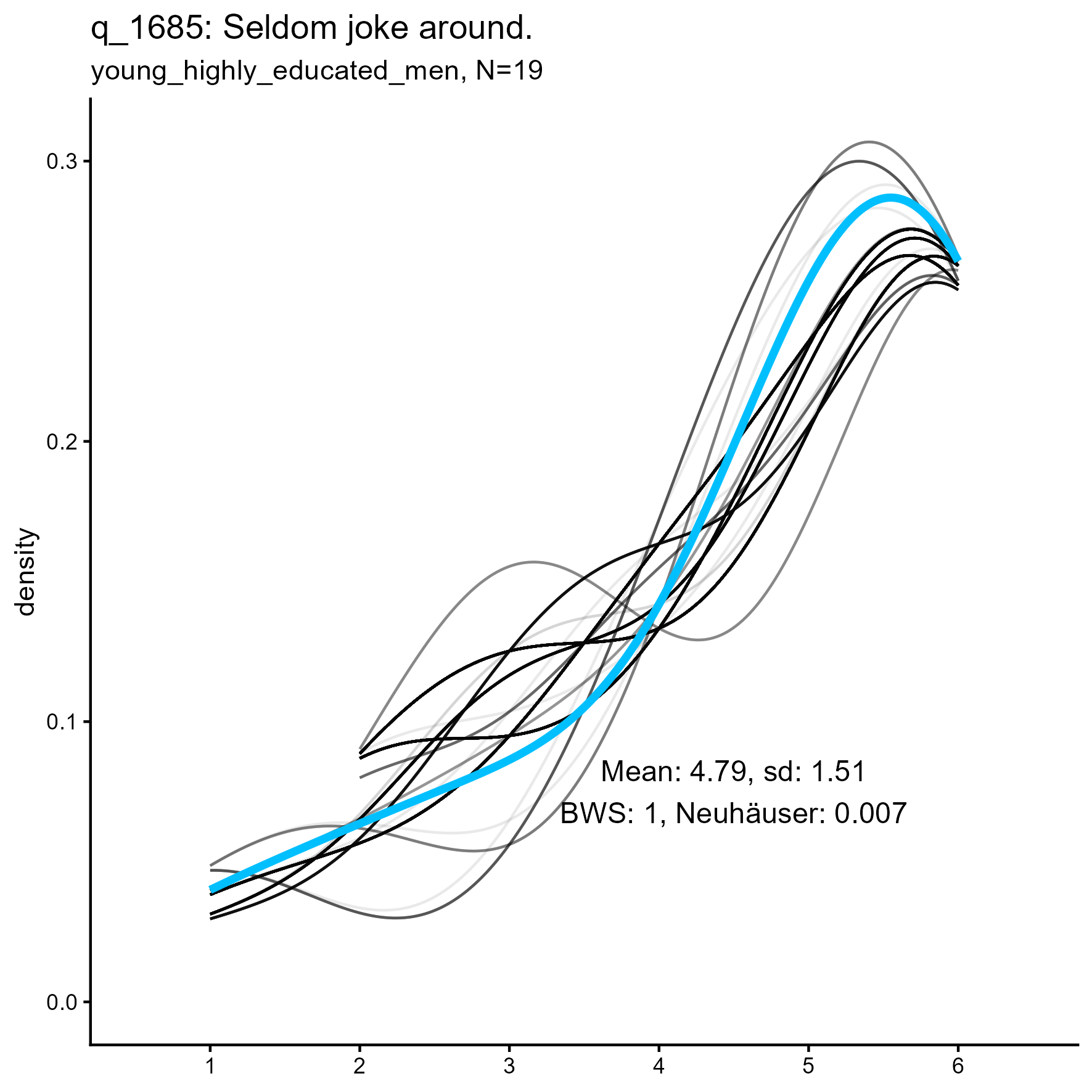
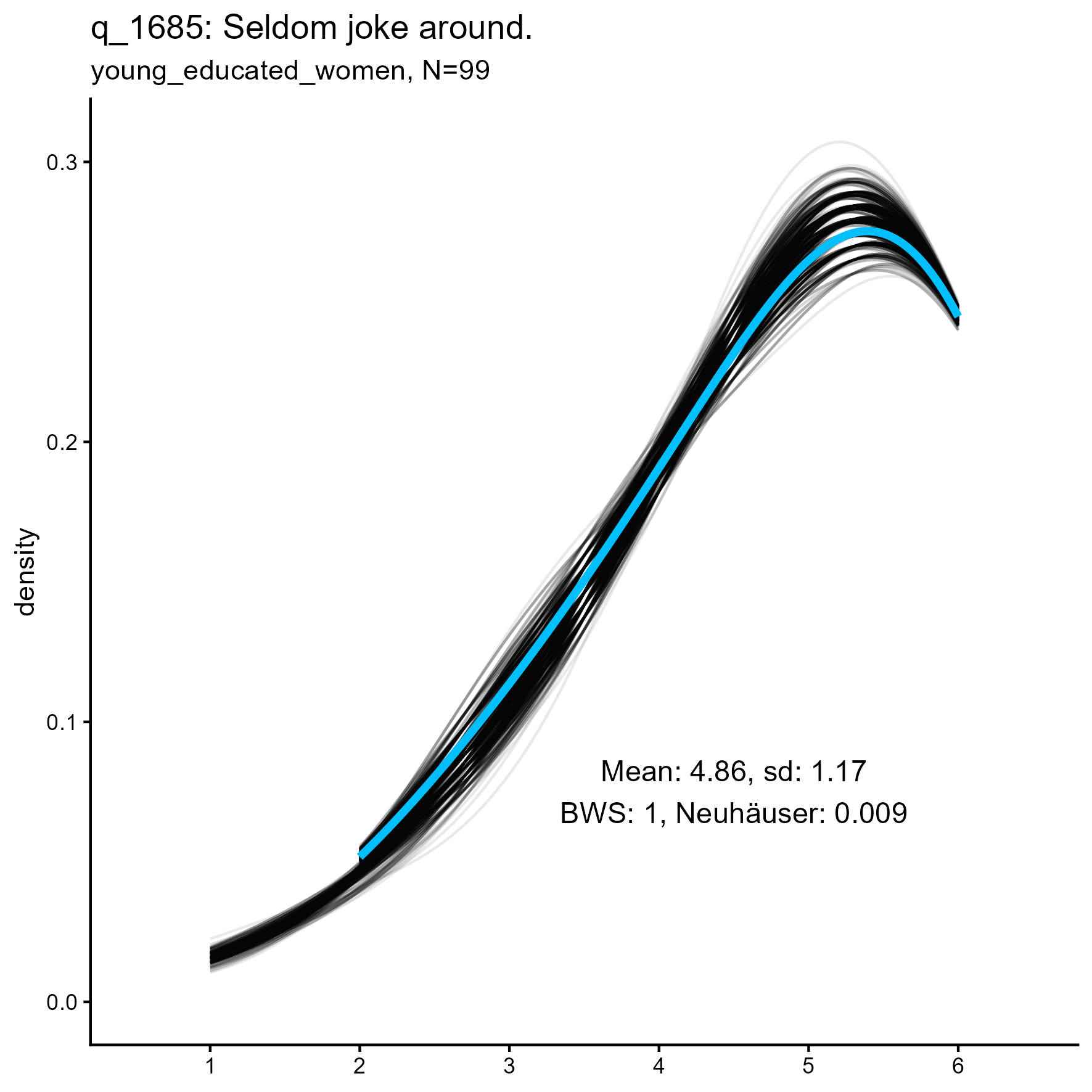
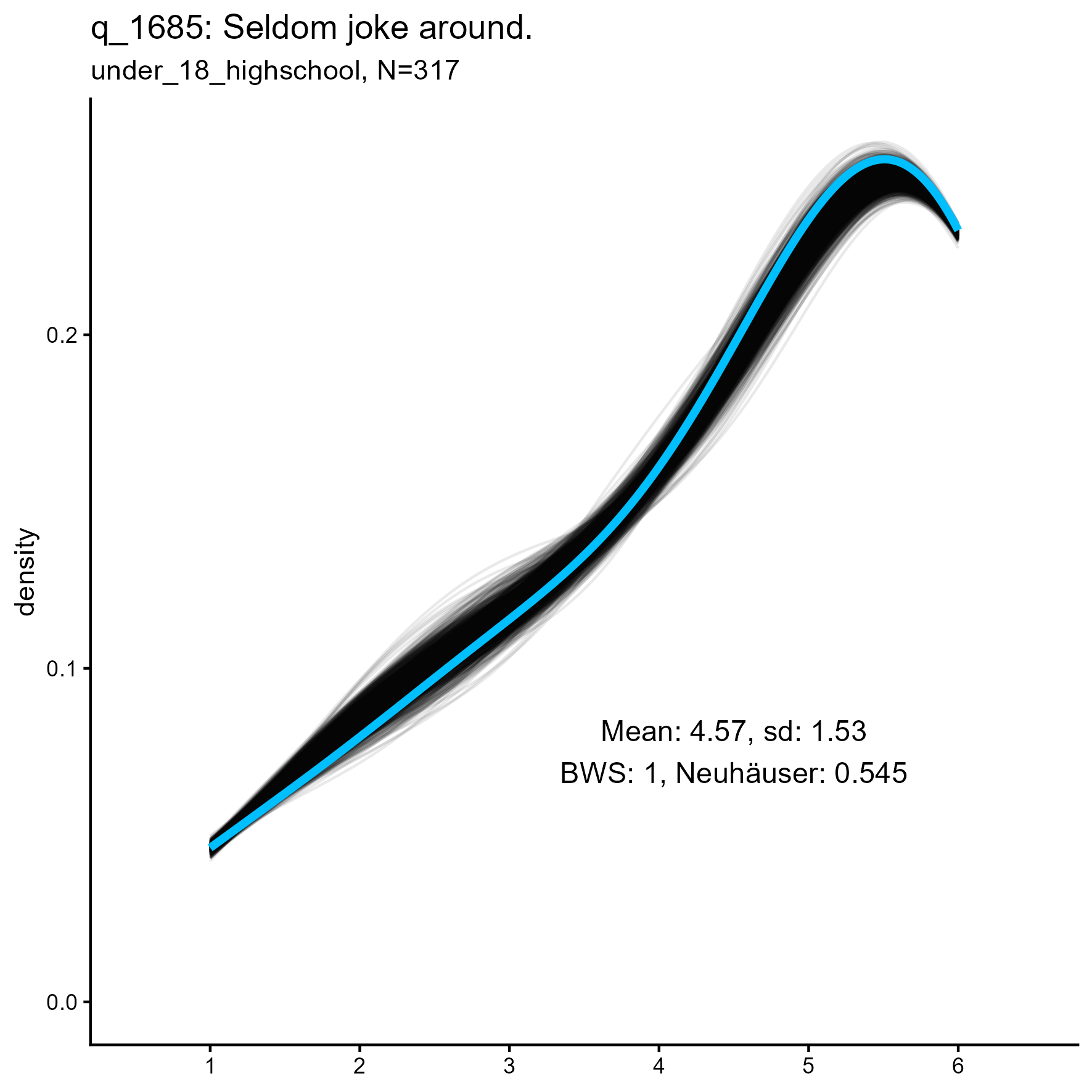
q_1685 ‘Seldom joke around’: Kernel Density plots for small, medium and large samples
q_1896 ‘Use others for my own ends’
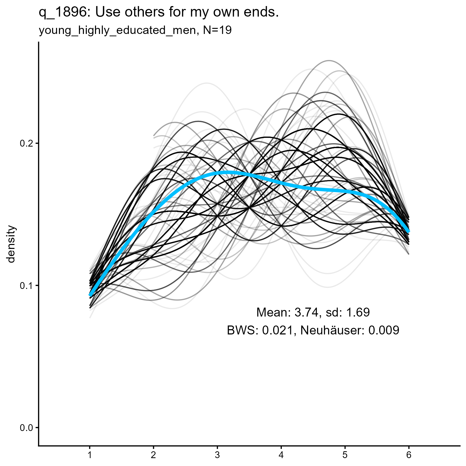
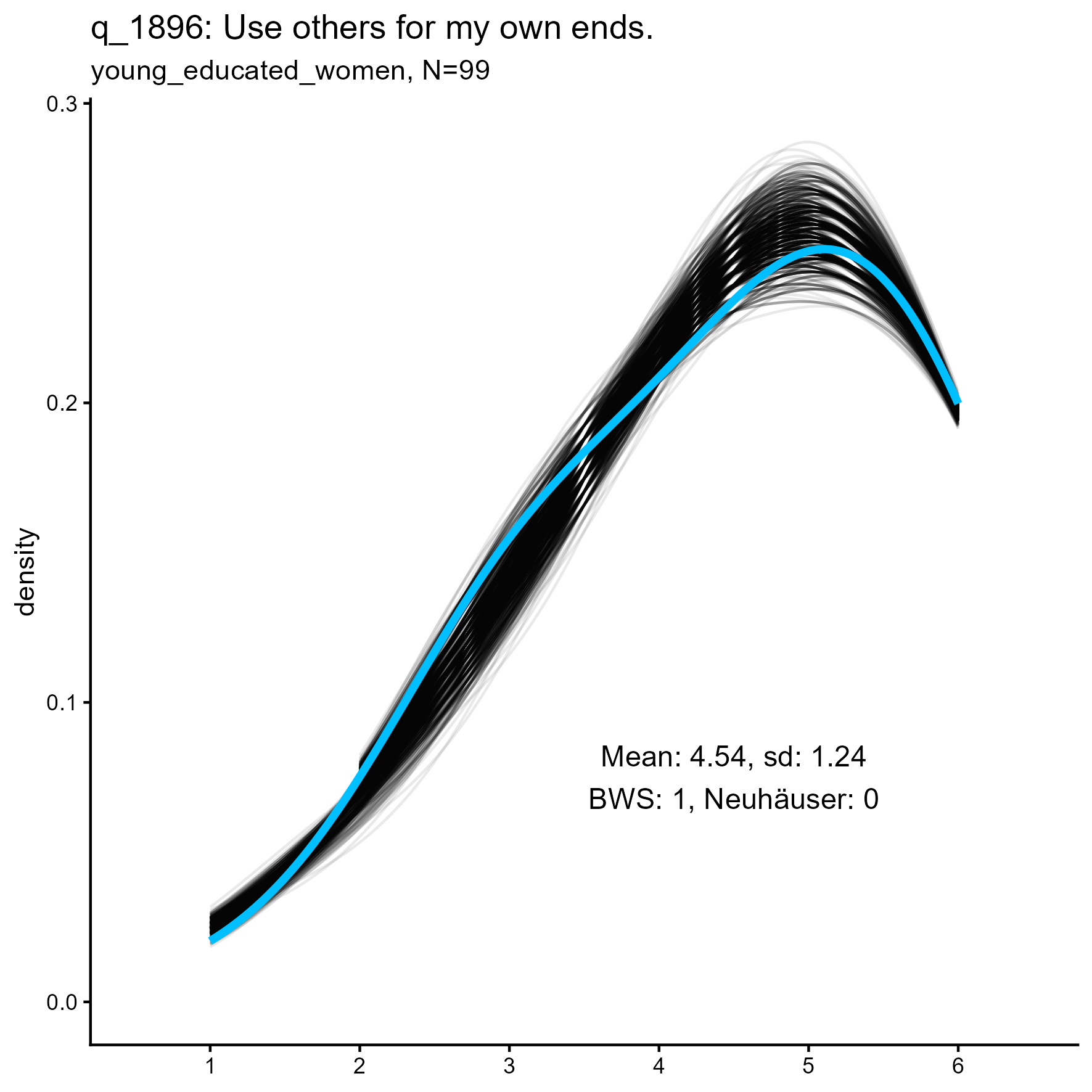
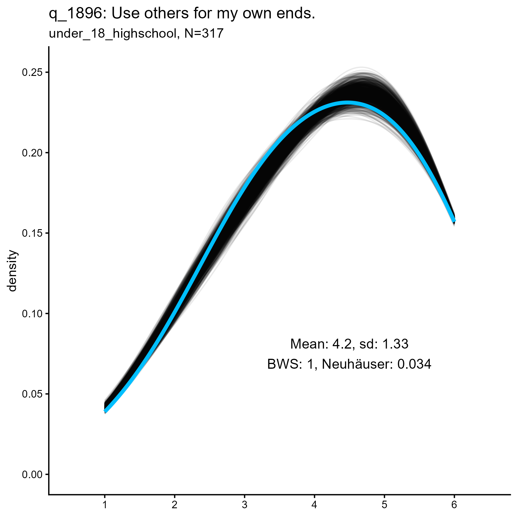
q_1058 ‘Use others for my own ends’: Kernel Density plots for small, medium and large samples
Summary Results
Results are much as we might expect:
Unimodal data are good, multimodal less so
Multimodal data are not well-represented by the
LikertMakeR::lfast() function, which consistently generates
unimodal data.
Larger sample sizes produce smoother unimodal data distributions
Original data in the very small sample size in the 19-subjects group frequently were multimodal, whereas original data from the medium-sized and large-sized groups were more often unimodal.
Appendix
Summary results for individual items
Rating scale items ranging from ‘1’ to ‘6’ from the SPI data set, for three samples of different sizes.
|
young men postgrad n=19 |
young women graduates n=99 |
under-18 highschool n=314 |
|
|---|---|---|---|
| q_253 | 1.000 / 0.021 | 1.000 / 0.003 | 1.000 / 0.003 |
| q_952 | 1.000 / 0.001 | 1.000 / 0.002 | 1.000 / 0.077 |
| q_1904 | 0.399 / 0.000 | 1.000 / 0.020 | 1.000 / 0.025 |
| q_578 | 1.000 / 0.002 | 1.000 / 0.009 | 1.000 / 0.026 |
| q_1367 | 1.000 / 0.000 | 1.000 / 0.013 | 1.000 / 0.026 |
| q_4252 | 0.185 / 0.001 | 1.000 / 0.025 | 1.000 / 0.283 |
| q_4296 | 1.000 / 0.001 | 1.000 / 0.010 | 1.000 / 0.073 |
| q_904 | 0.948 / 0.005 | 1.000 / 0.039 | 1.000 / 0.005 |
| q_240 | 1.000 / 0.000 | 1.000 / 0.001 | 1.000 / 0.062 |
| q_2745 | 1.000 / 0.008 | 1.000 / 0.011 | 1.000 / 0.036 |
| q_35 | 1.000 / 0.003 | 1.000 / 0.011 | 1.000 / 0.122 |
| q_565 | 0.662 / 0.003 | 1.000 / 0.008 | 1.000 / 0.058 |
| q_1201 | 1.000 / 0.000 | 1.000 / 0.033 | 1.000 / 0.070 |
| q_1624 | 0.094 / 0.001 | 1.000 / 0.000 | 1.000 / 0.013 |
| q_1045 | 1.000 / 0.006 | 1.000 / 0.084 | 1.000 / 0.119 |
| q_1855 | 1.000 / 0.000 | 1.000 / 0.027 | 1.000 / 0.077 |
| q_1243 | 1.000 / 0.075 | 1.000 / 0.019 | 1.000 / 0.170 |
| q_219 | 0.496 / 0.001 | 1.000 / 0.004 | 1.000 / 0.036 |
| q_610 | 1.000 / 0.001 | 1.000 / 0.040 | 1.000 / 0.535 |
| q_1389 | 1.000 / 0.000 | 1.000 / 0.009 | 1.000 / 0.002 |
| q_530 | 0.662 / 0.000 | 1.000 / 0.026 | 1.000 / 0.156 |
| q_56 | 0.351 / 0.001 | 1.000 / 0.024 | 1.000 / 0.083 |
| q_152 | 0.294 / 0.003 | 1.000 / 0.020 | 1.000 / 0.062 |
| q_566 | 1.000 / 0.001 | 1.000 / 0.012 | 1.000 / 0.010 |
| q_1329 | 1.000 / 0.002 | 1.000 / 0.024 | 1.000 / 0.007 |
| q_979 | 0.998 / 0.001 | 1.000 / 0.000 | 1.000 / 0.002 |
| q_345 | 1.000 / 0.000 | 1.000 / 0.000 | 1.000 / 0.015 |
| q_90 | 1.000 / 0.017 | 1.000 / 0.000 | 1.000 / 0.006 |
| q_1357 | 1.000 / 0.001 | 1.000 / 0.002 | 1.000 / 0.021 |
| q_312 | 0.823 / 0.000 | 1.000 / 0.011 | 1.000 / 0.004 |
| q_811 | 1.000 / 0.000 | 1.000 / 0.000 | 1.000 / 0.001 |
| q_1664 | 1.000 / 0.001 | 1.000 / 0.001 | 1.000 / 0.009 |
| q_1989 | 0.072 / 0.001 | 1.000 / 0.007 | 1.000 / 0.833 |
| q_1812 | 1.000 / 0.007 | 1.000 / 0.002 | 1.000 / 0.000 |
| q_1744 | 0.881 / 0.001 | 1.000 / 0.048 | 1.000 / 0.035 |
| q_1253 | 1.000 / 0.004 | 1.000 / 0.021 | 1.000 / 0.052 |
| q_128 | 1.000 / 0.000 | 1.000 / 0.014 | 1.000 / 0.103 |
| q_1173 | 1.000 / 0.000 | 1.000 / 0.021 | 1.000 / 0.043 |
| q_1027 | 0.284 / 0.000 | 1.000 / 0.011 | 1.000 / 0.058 |
| q_1254 | 1.000 / 0.000 | 1.000 / 0.001 | 1.000 / 0.000 |
| q_1867 | 0.664 / 0.002 | 1.000 / 0.000 | 1.000 / 0.004 |
| q_254 | 0.192 / 0.003 | 1.000 / 0.030 | 1.000 / 0.121 |
| q_4289 | 1.000 / 0.000 | 1.000 / 0.011 | 1.000 / 0.093 |
| q_1244 | 1.000 / 0.005 | 1.000 / 0.005 | 1.000 / 0.035 |
| q_1081 | 0.111 / 0.002 | 1.000 / 0.000 | 1.000 / 0.009 |
| q_348 | 1.000 / 0.000 | 1.000 / 0.007 | 1.000 / 0.241 |
| q_1738 | 1.000 / 0.096 | 1.000 / 0.028 | 1.000 / 0.000 |
| q_1915 | 0.067 / 0.000 | 1.000 / 0.007 | 1.000 / 0.089 |
| q_736 | 1.000 / 0.001 | 1.000 / 0.003 | 1.000 / 0.033 |
| q_1300 | 0.153 / 0.008 | 1.000 / 0.078 | 1.000 / 0.103 |
| q_689 | 1.000 / 0.031 | 1.000 / 0.056 | 1.000 / 0.031 |
| q_1281 | 1.000 / 0.000 | 1.000 / 0.041 | 1.000 / 0.014 |
| q_174 | 1.000 / 0.000 | 1.000 / 0.001 | 1.000 / 0.000 |
| q_660 | 1.000 / 0.000 | 1.000 / 0.000 | 1.000 / 0.013 |
| q_1763 | 1.000 / 0.014 | 1.000 / 0.160 | 1.000 / 0.002 |
| q_1683 | 0.228 / 0.006 | 1.000 / 0.053 | 1.000 / 0.099 |
| q_1923 | 1.000 / 0.003 | 1.000 / 0.005 | 1.000 / 0.000 |
| q_2765 | 1.000 / 0.014 | 1.000 / 0.021 | 1.000 / 0.102 |
| q_1781 | 0.308 / 0.000 | 1.000 / 0.066 | 1.000 / 0.113 |
| q_4249 | 0.110 / 0.003 | 1.000 / 0.012 | 1.000 / 0.042 |
| q_501 | 1.000 / 0.000 | 1.000 / 0.017 | 1.000 / 0.036 |
| q_1444 | 1.000 / 0.018 | 1.000 / 0.004 | 1.000 / 0.000 |
| q_493 | 1.000 / 0.000 | 1.000 / 0.009 | 1.000 / 0.039 |
| q_2754 | 1.000 / 0.036 | 1.000 / 0.009 | 1.000 / 0.120 |
| q_1424 | 0.851 / 0.010 | 1.000 / 0.062 | 1.000 / 0.076 |
| q_1416 | 0.275 / 0.009 | 1.000 / 0.010 | 1.000 / 0.003 |
| q_1483 | 0.729 / 0.003 | 1.000 / 0.013 | 1.000 / 0.000 |
| q_1609 | 0.958 / 0.001 | 1.000 / 0.015 | 1.000 / 0.000 |
| q_1242 | 1.000 / 0.027 | 1.000 / 0.011 | 1.000 / 0.147 |
| q_377 | 1.000 / 0.001 | 1.000 / 0.002 | 1.000 / 0.065 |
| q_1248 | 1.000 / 0.007 | 1.000 / 0.019 | 1.000 / 0.060 |
| q_803 | 1.000 / 0.000 | 1.000 / 0.011 | 1.000 / 0.100 |
| q_607 | 1.000 / 0.001 | 1.000 / 0.071 | 1.000 / 0.510 |
| q_755 | 1.000 / 0.000 | 1.000 / 0.005 | 1.000 / 0.141 |
| q_571 | 1.000 / 0.000 | 1.000 / 0.024 | 1.000 / 0.063 |
| q_1590 | 1.000 / 0.060 | 1.000 / 0.022 | 1.000 / 0.012 |
| q_1653 | 1.000 / 0.004 | 1.000 / 0.030 | 1.000 / 0.092 |
| q_39 | 1.000 / 0.018 | 1.000 / 0.031 | 1.000 / 0.061 |
| q_1052 | 0.684 / 0.003 | 1.000 / 0.059 | 1.000 / 0.077 |
| q_793 | 1.000 / 0.001 | 1.000 / 0.001 | 1.000 / 0.000 |
| q_1824 | 1.000 / 0.000 | 1.000 / 0.000 | 1.000 / 0.000 |
| q_851 | 1.000 / 0.015 | 1.000 / 0.003 | 1.000 / 0.025 |
| q_1585 | 0.248 / 0.032 | 1.000 / 0.038 | 1.000 / 0.017 |
| q_4243 | 0.061 / 0.007 | 1.000 / 0.022 | 1.000 / 0.121 |
| q_820 | 1.000 / 0.000 | 1.000 / 0.033 | 1.000 / 0.090 |
| q_598 | 0.502 / 0.001 | 1.000 / 0.051 | 1.000 / 0.065 |
| q_1505 | 1.000 / 0.039 | 1.000 / 0.030 | 1.000 / 0.021 |
| q_2853 | 0.906 / 0.001 | 1.000 / 0.000 | 1.000 / 0.001 |
| q_1452 | 0.579 / 0.000 | 1.000 / 0.007 | 1.000 / 0.018 |
| q_422 | 1.000 / 0.000 | 1.000 / 0.018 | 1.000 / 0.021 |
| q_1392 | 1.000 / 0.000 | 1.000 / 0.020 | 1.000 / 0.050 |
| q_4276 | 1.000 / 0.000 | 1.000 / 0.013 | 1.000 / 0.092 |
| q_1296 | 1.000 / 0.002 | 1.000 / 0.006 | 1.000 / 0.019 |
| q_1290 | 1.000 / 0.003 | 1.000 / 0.006 | 1.000 / 0.006 |
| q_369 | 0.354 / 0.000 | 1.000 / 0.034 | 1.000 / 0.068 |
| q_901 | 0.315 / 0.004 | 1.000 / 0.020 | 1.000 / 0.004 |
| q_379 | 0.817 / 0.044 | 1.000 / 0.040 | 1.000 / 0.089 |
| q_296 | 1.000 / 0.000 | 1.000 / 0.015 | 1.000 / 0.003 |
| q_1635 | 1.000 / 0.011 | 1.000 / 0.001 | 1.000 / 0.044 |
| q_612 | 1.000 / 0.003 | 1.000 / 0.002 | 1.000 / 0.230 |
| q_1880 | 1.000 / 0.206 | 1.000 / 0.223 | 1.000 / 0.006 |
| q_1694 | 1.000 / 0.033 | 1.000 / 0.016 | 1.000 / 0.012 |
| q_1462 | 1.000 / 0.041 | 1.000 / 0.000 | 1.000 / 0.000 |
| q_747 | 1.000 / 0.004 | 1.000 / 0.037 | 1.000 / 0.108 |
| q_1542 | 1.000 / 0.000 | 1.000 / 0.023 | 1.000 / 0.051 |
| q_1024 | 0.268 / 0.011 | 1.000 / 0.030 | 1.000 / 0.229 |
| q_797 | 0.118 / 0.008 | 1.000 / 0.008 | 1.000 / 0.000 |
| q_1825 | 1.000 / 0.000 | 1.000 / 0.000 | 1.000 / 0.000 |
| q_1832 | 0.947 / 0.001 | 1.000 / 0.008 | 1.000 / 0.072 |
| q_176 | 1.000 / 0.037 | 1.000 / 0.027 | 1.000 / 0.101 |
| q_684 | 1.000 / 0.000 | 1.000 / 0.002 | 1.000 / 0.002 |
| q_1371 | 1.000 / 0.000 | 1.000 / 0.009 | 1.000 / 0.163 |
| q_1662 | 1.000 / 0.001 | 1.000 / 0.005 | 1.000 / 0.024 |
| q_808 | 0.225 / 0.000 | 1.000 / 0.006 | 1.000 / 0.057 |
| q_1896 | 0.021 / 0.014 | 1.000 / 0.000 | 1.000 / 0.032 |
| q_1979 | 1.000 / 0.000 | 1.000 / 0.000 | 1.000 / 0.019 |
| q_1834 | 1.000 / 0.001 | 1.000 / 0.006 | 1.000 / 0.043 |
| q_1058 | 1.000 / 0.000 | 1.000 / 0.008 | 1.000 / 0.545 |
| q_4223 | 1.000 / 0.002 | 1.000 / 0.104 | 1.000 / 0.018 |
| q_1555 | 0.375 / 0.002 | 1.000 / 0.078 | 1.000 / 0.094 |
| q_169 | 0.245 / 0.000 | 1.000 / 0.009 | 1.000 / 0.034 |
| q_398 | 0.370 / 0.004 | 1.000 / 0.006 | 1.000 / 0.065 |
| q_131 | 1.000 / 0.000 | 1.000 / 0.004 | 1.000 / 0.015 |
| q_871 | 0.802 / 0.000 | 1.000 / 0.020 | 1.000 / 0.085 |
| q_1685 | 1.000 / 0.005 | 1.000 / 0.009 | 1.000 / 0.548 |
| q_1706 | 1.000 / 0.005 | 1.000 / 0.035 | 1.000 / 0.059 |
| q_1132 | 1.000 / 0.001 | 1.000 / 0.010 | 1.000 / 0.042 |
| q_1310 | 1.000 / 0.000 | 1.000 / 0.013 | 1.000 / 0.192 |
| q_142 | 0.546 / 0.001 | 1.000 / 0.033 | 1.000 / 0.114 |
| q_1461 | 0.645 / 0.002 | 1.000 / 0.016 | 1.000 / 0.013 |
| q_2005 | 1.000 / 0.002 | 1.000 / 0.003 | 1.000 / 0.000 |
| q_1303 | 1.000 / 0.074 | 1.000 / 0.045 | 1.000 / 0.012 |
| q_1280 | 1.000 / 0.008 | 1.000 / 0.022 | 1.000 / 0.075 |
| q_1840 | 0.188 / 0.000 | 1.000 / 0.017 | 1.000 / 0.027 |
| q_1328 | 1.000 / 0.000 | 1.000 / 0.004 | 1.000 / 0.014 |